Tutorial about radial distance distribution analysis

The pairwise distance distribution p(r) - as derived from a histogram of pairwise distances - represents the probability distribution function to find for a localization at r = 0 another localization at distance r + delta_r.

The radial distribution function (also called pair correlation function) g(r) represents the pairwise distance distribution function p(r) normalized to the region measure of the circular ring or shell with inner radius r and outer radius r + delta_r and relative to the expected number of localizations per unit area for complete spatial randomness.

from pathlib import Path

%matplotlib inline

import numpy as np
import matplotlib.pyplot as plt

import locan as lc

lc.show_versions(system=False, dependencies=False, verbose=False)

Locan:
   version: 0.22.0.dev32+g4bfc3ab8b

Python:
   version: 3.11.14

rng = np.random.default_rng(seed=1)

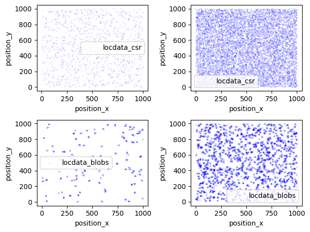
Synthetic data

We simulate localization data at two different intensities (localization density) that is (i) homogeneously Poisson distributed (also described as complete spatial randomness, csr) and that (ii) follows a Neyman-Scott distribution (blobs).

locdata_csr_0 = lc.simulate_Poisson(intensity=1e-3, region=((0,1000), (0,1000)), seed=rng)
locdata_csr_1 = lc.simulate_Poisson(intensity=1e-2, region=((0,1000), (0,1000)), seed=rng)

Jupyter environment detected. Enabling Open3D WebVisualizer.
[Open3D INFO] WebRTC GUI backend enabled.
[Open3D INFO] WebRTCWindowSystem: HTTP handshake server disabled.

locdata_blob_0 = lc.simulate_Thomas(parent_intensity=1e-4, region=((0, 1000), (0, 1000)), cluster_mu=10, cluster_std=5, seed=rng)
locdata_blob_1 = lc.simulate_Thomas(parent_intensity=1e-3, region=((0, 1000), (0, 1000)), cluster_mu=10, cluster_std=5, seed=rng)

print("Number of localizations:")
print("csr_0:", len(locdata_csr_0))
print("csr_1:", len(locdata_csr_1))
print("blob_0:", len(locdata_blob_0))
print("blob_1:", len(locdata_blob_1))

Number of localizations:
csr_0: 1001
csr_1: 10082
blob_0: 1080
blob_1: 10151

Scatter plot

fig, axes = plt.subplots(nrows=2, ncols=2)
locdata_csr_0.data.plot.scatter(x='position_x', y='position_y', ax=axes[0, 0], color='Blue', s=1, alpha=0.1, label='locdata_csr')
locdata_csr_1.data.plot.scatter(x='position_x', y='position_y', ax=axes[0, 1], color='Blue', s=1, alpha=0.1, label='locdata_csr')
locdata_blob_0.data.plot.scatter(x='position_x', y='position_y', ax=axes[1, 0], color='Blue', s=1, alpha=0.1, label='locdata_blobs')
locdata_blob_1.data.plot.scatter(x='position_x', y='position_y', ax=axes[1, 1], color='Blue', s=1, alpha=0.1, label='locdata_blobs')
plt.tight_layout()
plt.show()

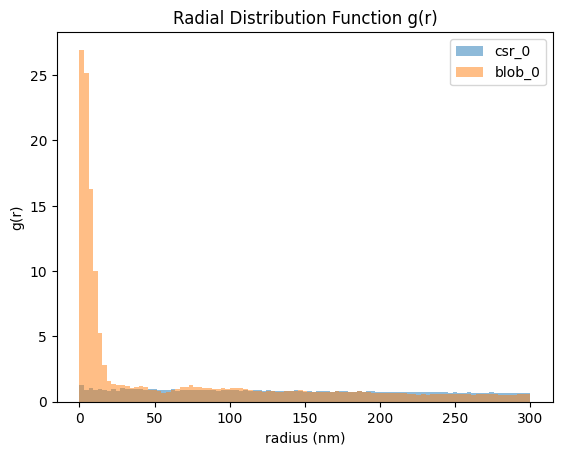
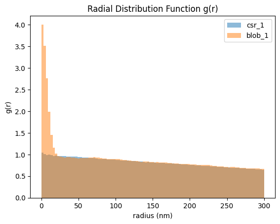
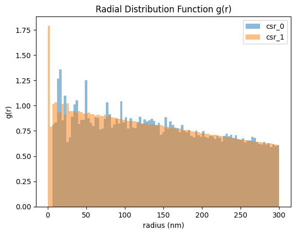
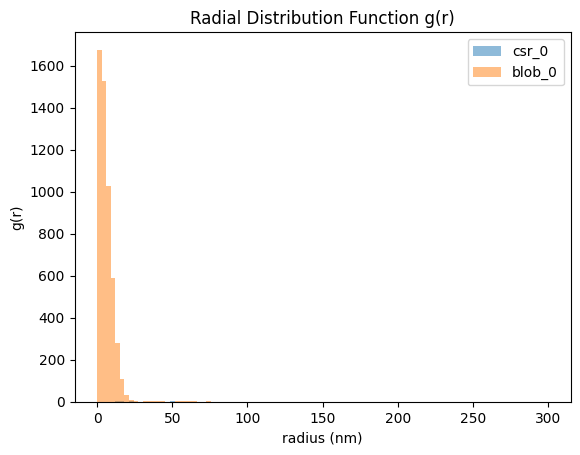
Radial distance distribution

We determine all pairwise distances and the normalized radial distance distribution (resembling the pair correlation function).

bins = np.linspace(0, 300, 100)
rdf_csr_0 = lc.RadialDistribution(bins=bins).compute(locdata_csr_0)
rdf_csr_1 = lc.RadialDistribution(bins=bins).compute(locdata_csr_1)
rdf_blob_0 = lc.RadialDistribution(bins=bins).compute(locdata_blob_0)
rdf_blob_1 = lc.RadialDistribution(bins=bins).compute(locdata_blob_1)

rdf_csr_0.hist(alpha=0.5, label="csr_0")
rdf_blob_0.hist(alpha=0.5, label="blob_0");

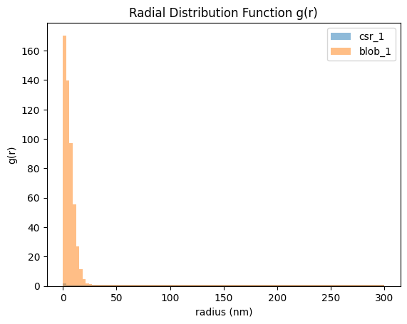
rdf_csr_1.hist(alpha=0.5, label="csr_1")
rdf_blob_1.hist(alpha=0.5, label="blob_1");

Synthetic data - 3D

locdata_csr_0 = lc.simulate_Poisson(intensity=1e-6, region=((0,1000), (0,1000), (0,1000)), seed=rng)
locdata_csr_1 = lc.simulate_Poisson(intensity=1e-5, region=((0,1000), (0,1000), (0,1000)), seed=rng)

locdata_blob_0 = lc.simulate_Thomas(parent_intensity=1e-7, region=((0, 1000), (0, 1000), (0,1000)), cluster_mu=10, cluster_std=5, seed=rng)
locdata_blob_1 = lc.simulate_Thomas(parent_intensity=1e-6, region=((0, 1000), (0, 1000), (0,1000)), cluster_mu=10, cluster_std=5, seed=rng)

print("Number of localizations:")
print("csr_0:", len(locdata_csr_0))
print("csr_1:", len(locdata_csr_1))
print("blob_0:", len(locdata_blob_0))
print("blob_1:", len(locdata_blob_1))

Number of localizations:
csr_0: 1054
csr_1: 9785
blob_0: 971
blob_1: 10279

We determine all pairwise distances and normalized radial distance distribution (resembling the pair correlation function).

bins = np.linspace(0, 300, 100)
rdf_csr_0 = lc.RadialDistribution(bins=bins).compute(locdata_csr_0)
rdf_csr_1 = lc.RadialDistribution(bins=bins).compute(locdata_csr_1)
rdf_blob_0 = lc.RadialDistribution(bins=bins).compute(locdata_blob_0)
rdf_blob_1 = lc.RadialDistribution(bins=bins).compute(locdata_blob_1)

rdf_csr_0.hist(alpha=0.5, label="csr_0")
rdf_csr_1.hist(alpha=0.5, label="csr_1");

rdf_csr_0.hist(alpha=0.5, label="csr_0")
rdf_blob_0.hist(alpha=0.5, label="blob_0");

rdf_csr_1.hist(alpha=0.5, label="csr_1")
rdf_blob_1.hist(alpha=0.5, label="blob_1");

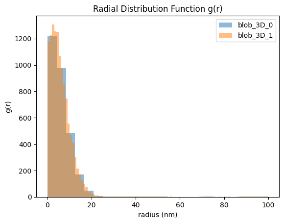
Radial distance distribution with precomputed distances

You can use precomputed pairwise distances for quick variation of bin (radii) settings.

locdata_blob_3D = lc.simulate_Thomas(parent_intensity=1e-7, region=((0, 1000), (0, 1000), (0, 1000)), cluster_mu=10, cluster_std=5, seed=rng)
locdata_blob_3D.print_summary()

identifier: "9"
comment: ""
source: SIMULATION
state: RAW
element_count: 1252
frame_count: 0
creation_time {
  2026-04-30T08:35:58.189012Z
}

pd_blob_3D = lc.PairDistances().compute(locdata_blob_3D)
pd_blob_3D.results.describe()

	pair_distance
count	783126.000000
mean	639.661716
std	247.977636
min	0.478555
25%	463.858376
50%	639.817439
75%	818.012399
max	1435.665071

bins = np.linspace(0, 100, 25)
rdf_blob_3D_0 = lc.RadialDistribution(bins=bins, pair_distances=pd_blob_3D).compute(locdata_blob_3D)
bins = np.linspace(0, 100, 100)
rdf_blob_3D_1 = lc.RadialDistribution(bins=bins, pair_distances=pd_blob_3D).compute(locdata_blob_3D)

rdf_blob_3D_0.hist(alpha=0.5, label="blob_3D_0")
rdf_blob_3D_1.hist(alpha=0.5, label="blob_3D_1");

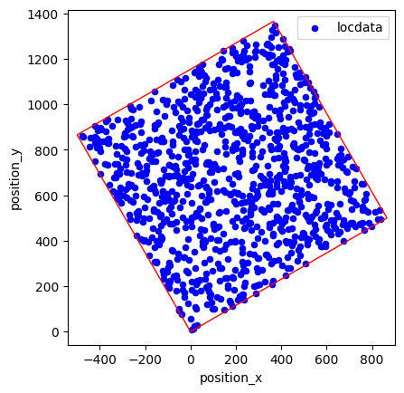
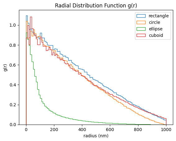
Radial distribution function for various regions

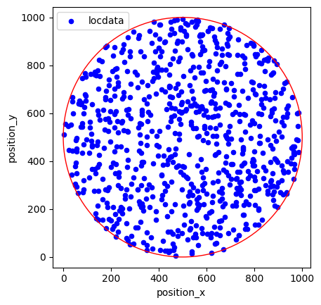
We compare radial distribution functions for localizations homogeneously distributed in bounded regions.

bins = np.linspace(0, 1000, 100)

region_rectangle = lc.Rectangle((0, 0), 1000, 1000, 30)
locdata_rectangle = lc.simulate_Poisson(intensity=1e-3, region=region_rectangle, seed=rng)
rdf_rectangle = lc.RadialDistribution(bins=bins).compute(locdata=locdata_rectangle)

fig, ax = plt.subplots(nrows=1, ncols=1)
locdata_rectangle.data.plot.scatter(x='position_x', y='position_y', ax=ax, color='Blue', label='locdata')
locdata_rectangle.region.plot(ax=ax, fill=False, color='Red')
ax.set_aspect("equal")
plt.show()

region_circle = lc.Ellipse((500, 500), 1000, 1000, 0)
locdata_circle = lc.simulate_Poisson(intensity=1e-3, region=region_circle, seed=rng)
rdf_circle = lc.RadialDistribution(bins=bins).compute(locdata=locdata_circle)

fig, ax = plt.subplots(nrows=1, ncols=1)
locdata_circle.data.plot.scatter(x='position_x', y='position_y', ax=ax, color='Blue', label='locdata')
locdata_circle.region.plot(ax=ax, fill=False, color='Red')
ax.set_aspect("equal")
plt.show()

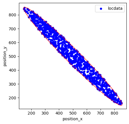
region_ellipse = lc.Ellipse((500, 500), 100, 1000, 45)
locdata_ellipse = lc.simulate_Poisson(intensity=1e-2, region=region_ellipse, seed=rng)
rdf_ellipse = lc.RadialDistribution(bins=bins).compute(locdata=locdata_ellipse)

fig, ax = plt.subplots(nrows=1, ncols=1)
locdata_ellipse.data.plot.scatter(x='position_x', y='position_y', ax=ax, color='Blue', label='locdata')
locdata_ellipse.region.plot(ax=ax, fill=False, color='Red');
ax.set_aspect("equal")
plt.show()

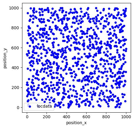
region_cuboid = lc.AxisOrientedCuboid((0, 0, 0), 1000, 1000, 1000)
locdata_cuboid = lc.simulate_Poisson(intensity=1e-6, region=region_cuboid, seed=rng)
rdf_cuboid = lc.RadialDistribution(bins=bins).compute(locdata=locdata_cuboid)

fig, ax = plt.subplots(nrows=1, ncols=1)
locdata_cuboid.data.plot.scatter(x='position_x', y='position_y', ax=ax, color='Blue', label='locdata')
#locdata_cuboid.region.plot(ax=ax, fill=False, color='Red');
ax.set_aspect("equal")
plt.show()

rdf_rectangle.hist(label="rectangle", histtype="step")
rdf_circle.hist(label="circle", histtype="step")
rdf_ellipse.hist(label="ellipse", histtype="step")
rdf_cuboid.hist(label="cuboid", histtype="step");

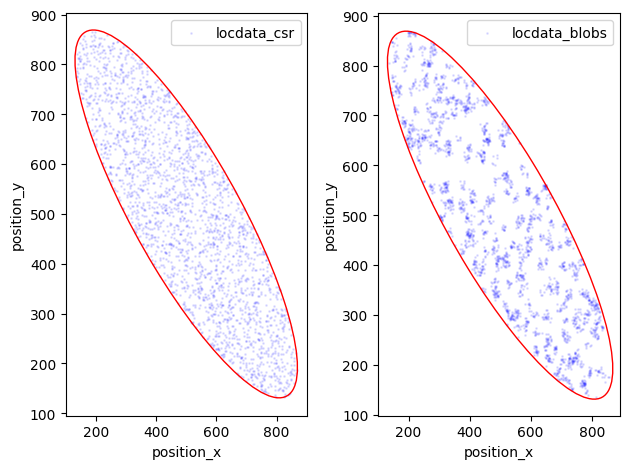
Radial distribution function normalized for specific regions of interest

To correct for boundary effects from the enclosing region, compute a radial distance distribution relative to that of a homogeneous point process in the same region.

region_ellipse = lc.Ellipse((500, 500), 300, 1000, 45)

locdata_csr = lc.simulate_Poisson(intensity=1e-2, region=region_ellipse, seed=rng)
locdata_blobs = lc.simulate_Thomas(parent_intensity=1e-3, region=region_ellipse, cluster_mu=10, cluster_std=5, seed=rng)

fig, axes = plt.subplots(nrows=1, ncols=2)
locdata_csr.data.plot.scatter(x='position_x', y='position_y', ax=axes[0], color='Blue', s=1, alpha=0.1, label='locdata_csr')
locdata_csr.region.plot(ax=axes[0], fill=False, color='Red')
locdata_blobs.data.plot.scatter(x='position_x', y='position_y', ax=axes[1], color='Blue', s=1, alpha=0.1, label='locdata_blobs')
locdata_blobs.region.plot(ax=axes[1], fill=False, color='Red')
plt.tight_layout()
plt.show()

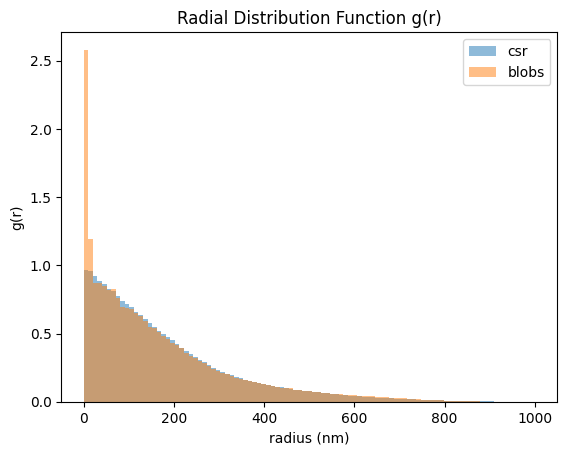
bins = np.linspace(0, 1000, 100)
rdf_csr = lc.RadialDistribution(bins=bins).compute(locdata=locdata_csr)
rdf_blobs = lc.RadialDistribution(bins=bins).compute(locdata=locdata_blobs)

rdf_csr.hist(alpha=0.5, label="csr")
rdf_blobs.hist(alpha=0.5, label="blobs");

Create a new RadialDistribution instance to carry the relative data.

results_corrected = lc.RadialDistributionResults()
results_corrected.radii = rdf_blobs.results.radii
results_corrected.data = rdf_blobs.results.data / rdf_csr.results.data

rdf = lc.RadialDistribution()
rdf.results = results_corrected

---------------------------------------------------------------------------
TypeError                                 Traceback (most recent call last)
Cell In[38], line 1
----> 1 rdf = lc.RadialDistribution()
      2 rdf.results = results_corrected

TypeError: RadialDistribution.__init__() missing 1 required positional argument: 'bins'

rdf.hist(label="blobs vs csr");

The peak at small radii represents the cluster.

bins = np.linspace(0, 100, 100)
rdf_csr = lc.RadialDistribution(bins=bins).compute(locdata=locdata_csr)
rdf_blobs = lc.RadialDistribution(bins=bins).compute(locdata=locdata_blobs)

rdf_csr.hist(alpha=0.5, label="csr")
rdf_blobs.hist(alpha=0.5, label="blobs");