Tutorial about rendering LocData
from pathlib import Path

%matplotlib inline
# %matplotlib widget

import numpy as np
import pandas as pd
import matplotlib.pyplot as plt
from mpl_toolkits.mplot3d import Axes3D

import locan as lc
lc.show_versions(system=False, dependencies=False, verbose=False)
Locan:
   version: 0.22.0.dev32+g4bfc3ab8b

Python:
   version: 3.11.14
Synthetic data
Localizations are simulated that are distributed according to a Neyman-Scott distribution (blobs).
rng = np.random.default_rng(seed=1)
locdata = lc.simulate_Thomas(parent_intensity=1e-5, region=((0, 1000), (0, 1000)), cluster_mu=100, cluster_std=10, seed=rng)

locdata.print_summary()
Jupyter environment detected. Enabling Open3D WebVisualizer.
[Open3D INFO] WebRTC GUI backend enabled.
[Open3D INFO] WebRTCWindowSystem: HTTP handshake server disabled.
identifier: "1"
comment: ""
source: SIMULATION
state: RAW
element_count: 705
frame_count: 0
creation_time {
  2026-04-30T08:38:30.745328Z
}
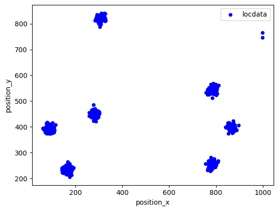
Since localization data is kept as a pandas dataframe standard plotting routines from pandas or matplotlip can be used.
fig, ax = plt.subplots(nrows=1, ncols=1)
locdata.data.plot.scatter(x='position_x', y='position_y', ax=ax, color='Blue', label='locdata')
plt.show()
Render by simple 2D binning
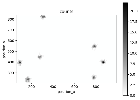
A method for simply binning localization data in 2D pixels is provided.
img, bins, label = lc.histogram(locdata, bin_size=10)
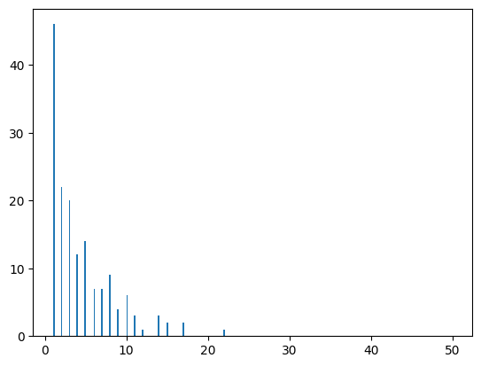
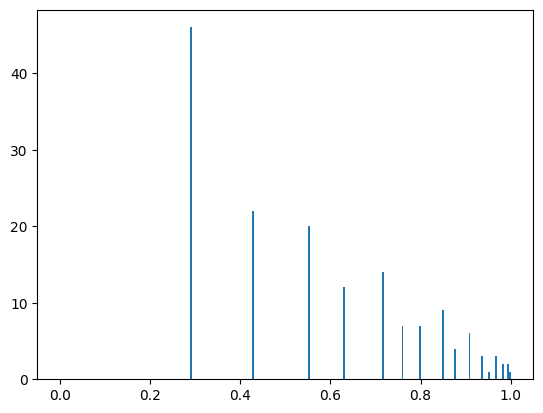
The intensity values of the binned locdata are distributed as:
plt.hist(img.ravel(), bins=256, range=(1, 50), fc='k', ec='k');
The intensity values can be rescaled in many ways. There are normalization classes and a convenience function in the locan.render.transformation module with predefined transformations as listed in locan.Trafo:
list(lc.Trafo)
[<Trafo.NONE: 0>,
 <Trafo.STANDARDIZE: 1>,
 <Trafo.STANDARDIZE_UINT8: 2>,
 <Trafo.ZERO: 3>,
 <Trafo.ZERO_UINT8: 4>,
 <Trafo.EQUALIZE: 5>,
 <Trafo.EQUALIZE_UINT8: 6>,
 <Trafo.EQUALIZE_ALL: 7>,
 <Trafo.EQUALIZE_ALL_UINT8: 8>,
 <Trafo.EQUALIZE_0P3: 9>,
 <Trafo.EQUALIZE_0P3_UINT8: 10>,
 <Trafo.EQUALIZE_0P3_ALL: 11>,
 <Trafo.EQUALIZE_0P3_ALL_UINT8: 12>]
img_new = lc.adjust_contrast(img, rescale=lc.Trafo.STANDARDIZE)
epsilon = np.finfo(float).resolution
plt.hist(img_new.ravel(), bins=256, range=(epsilon, 1), fc='k', ec='k');
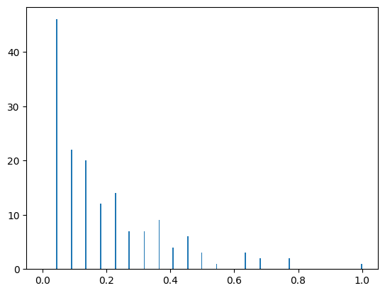
norm = lc.HistogramEqualization(power=1, mask=img>0)
img_new = norm(img)
plt.hist(img_new.ravel(), bins=256, range=(epsilon, 1), fc='k', ec='k');
The render_2d method can directly provide a new figure as output.
lc.render_2d(locdata, bin_size=10);
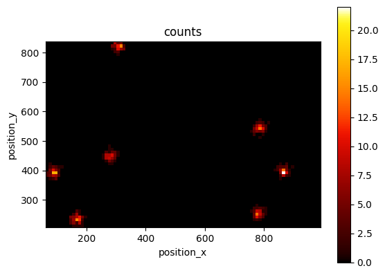
Or it can be used within the matplotlib environment.
fig, ax = plt.subplots(nrows=1, ncols=1)
lc.render_2d(locdata, ax = ax, bin_size=10, cmap='viridis')
plt.show()
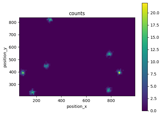
Intensity is per default scaled to the min and max intensity values but can be rescaled by applying any norm function as described for matplotlib.imshow:
norm = plt.Normalize(vmax=10)
lc.render_2d(locdata, bin_size=10, norm=norm);
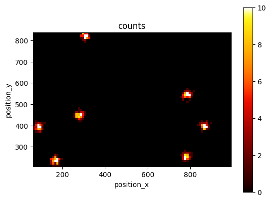
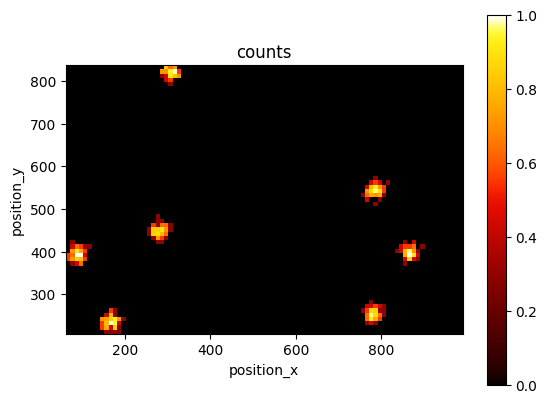
Intensity can also be rescaled by normalization functions as defined in locan.Trafo. Histogram equlization yields this image:
lc.render_2d(locdata, bin_size=10, rescale=lc.Trafo.EQUALIZE);
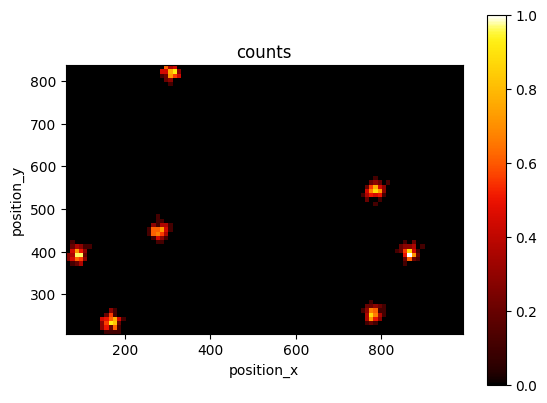
Histogram equlization with a power-intensification of p=0.3 yields this image:
lc.render_2d(locdata, bin_size=10, rescale=lc.Trafo.EQUALIZE_0P3);
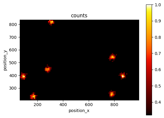
Any callable normalization object can be passed into the rescale kwarg:
norm = lc.HistogramEqualization(power=0.3)
lc.render_2d(locdata, bin_size=10, rescale=norm);
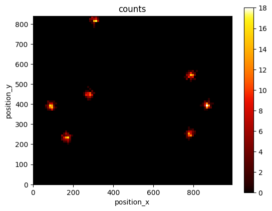
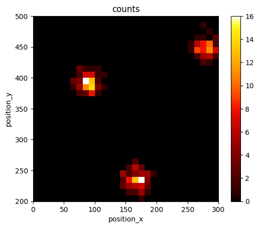
The image size is set automatically to the min and max coordinates but can be set to (0, max) or an arbitrary range.
lc.render_2d(locdata, bin_size=10, bin_range='zero');
lc.render_2d(locdata, bin_size=10, bin_range=((0, 300),(200, 500)));
Use different libraries for rendering
Rendering can also be carried out with a different render engine. Choose one of the following (MPL is the standard matplotlib):
list(lc.RenderEngine)
[<RenderEngine.MPL: 0>,
 <RenderEngine.MPL_SCATTER_DENSITY: 1>,
 <RenderEngine.NAPARI: 2>]
napari
As external viewer you can use napari.
or alternatively:
Choose colormaps
Colormaps can be chosen in matplotlib, napari and other visualization tools.
Colormaps are identified through specific class instances or by a name.
locan.Colormap serves as adapter class for the various visualization tools.
A Colormap instance can be created with the get_colormap function:
colormap = lc.get_colormap("viridis")
colormap.name
'viridis'
colormap.matplotlib

A mapping of names on Colormap instances is provided and can be extended by users. If a colormap name is provided to any rendering function, first the colormap_registry is searched, then the maplotlib registry and finally napari colormap names.
lc.colormap_registry
{'cet_fire': <locan.visualize.colormap.Colormap at 0x7dadd8be3cd0>,
 'cet_fire_r': <locan.visualize.colormap.Colormap at 0x7dadd8a13950>,
 'cet_gray': <locan.visualize.colormap.Colormap at 0x7dadd8a13910>,
 'cet_gray_r': <locan.visualize.colormap.Colormap at 0x7dadd8a3be90>,
 'cet_coolwarm': <locan.visualize.colormap.Colormap at 0x7dadd8a3be50>,
 'cet_glasbey_dark': <locan.visualize.colormap.Colormap at 0x7dadd8a3bed0>,
 'viridis': <locan.visualize.colormap.Colormap at 0x7dadd8a3bfd0>,
 'viridis_r': <locan.visualize.colormap.Colormap at 0x7dadd8a400d0>,
 'gray': <locan.visualize.colormap.Colormap at 0x7dadd8a40190>,
 'gray_r': <locan.visualize.colormap.Colormap at 0x7dadd8a40250>,
 'turbo': <locan.visualize.colormap.Colormap at 0x7dadd8a40310>,
 'coolwarm': <locan.visualize.colormap.Colormap at 0x7dadd8a403d0>,
 'tab20': <locan.visualize.colormap.Colormap at 0x7dadd8a40490>}
Default colormaps are defined for use with locan and can be accessed through a mapping or an enum:
lc.COLORMAP_DEFAULTS
{'CONTINUOUS': 'cet_fire',
 'CONTINUOUS_REVERSE': 'cet_fire_r',
 'CONTINUOUS_GRAY': 'cet_gray',
 'CONTINUOUS_GRAY_REVERSE': 'cet_gray_r',
 'DIVERGING': 'cet_coolwarm',
 'CATEGORICAL': 'cet_glasbey_dark',
 'TURBO': 'turbo'}
list(lc.Colormaps)
[<Colormaps.CONTINUOUS: 'cet_fire'>,
 <Colormaps.CONTINUOUS_REVERSE: 'cet_fire_r'>,
 <Colormaps.CONTINUOUS_GRAY: 'cet_gray'>,
 <Colormaps.CONTINUOUS_GRAY_REVERSE: 'cet_gray_r'>,
 <Colormaps.DIVERGING: 'cet_coolwarm'>,
 <Colormaps.CATEGORICAL: 'cet_glasbey_dark'>,
 <Colormaps.TURBO: 'turbo'>]
lc.render_2d(locdata, bin_size=10, cmap=lc.Colormaps.CONTINUOUS_GRAY_REVERSE);