Tutorial about pairwise distance analysis

The pairwise distance distribution p(r) - as derived from a histogram of pairwise distances - represents the probability distribution function to find for a localization at r = 0 another localization at distance r + delta_r.

from pathlib import Path

%matplotlib inline

import numpy as np
import matplotlib.pyplot as plt

import locan as lc

lc.show_versions(system=False, dependencies=False, verbose=False)

Locan:
   version: 0.22.0.dev32+g4bfc3ab8b

Python:
   version: 3.11.14

rng = np.random.default_rng(seed=1)

Synthetic data

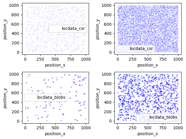
We simulate localization data at two different intensities (localization density) that is (i) homogeneously Poisson distributed (also described as complete spatial randomness, csr) and that (ii) follows a Neyman-Scott distribution (blobs).

locdata_csr_0 = lc.simulate_Poisson(intensity=1e-3, region=((0,1000), (0,1000)), seed=rng)
locdata_csr_1 = lc.simulate_Poisson(intensity=1e-2, region=((0,1000), (0,1000)), seed=rng)

Jupyter environment detected. Enabling Open3D WebVisualizer.
[Open3D INFO] WebRTC GUI backend enabled.
[Open3D INFO] WebRTCWindowSystem: HTTP handshake server disabled.

locdata_blob_0 = lc.simulate_Thomas(parent_intensity=1e-4, region=((0, 1000), (0, 1000)), cluster_mu=10, cluster_std=5, seed=rng)
locdata_blob_1 = lc.simulate_Thomas(parent_intensity=1e-3, region=((0, 1000), (0, 1000)), cluster_mu=10, cluster_std=5, seed=rng)

print("Number of localizations:")
print("csr_0:", len(locdata_csr_0))
print("csr_1:", len(locdata_csr_1))
print("blob_0:", len(locdata_blob_0))
print("blob_1:", len(locdata_blob_1))

Number of localizations:
csr_0: 1001
csr_1: 10082
blob_0: 1080
blob_1: 10151

Scatter plot

fig, axes = plt.subplots(nrows=2, ncols=2)
locdata_csr_0.data.plot.scatter(x='position_x', y='position_y', ax=axes[0, 0], color='Blue', s=1, alpha=0.1, label='locdata_csr')
locdata_csr_1.data.plot.scatter(x='position_x', y='position_y', ax=axes[0, 1], color='Blue', s=1, alpha=0.1, label='locdata_csr')
locdata_blob_0.data.plot.scatter(x='position_x', y='position_y', ax=axes[1, 0], color='Blue', s=1, alpha=0.1, label='locdata_blobs')
locdata_blob_1.data.plot.scatter(x='position_x', y='position_y', ax=axes[1, 1], color='Blue', s=1, alpha=0.1, label='locdata_blobs')
plt.tight_layout()
plt.show()

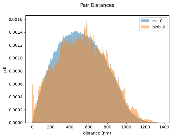
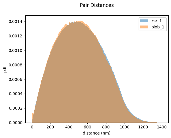
Pairwise distances

We determine all pairwise distances and plot the pair distance probability distribution.

pd_csr_0 = lc.PairDistances().compute(locdata_csr_0)
pd_csr_1 = lc.PairDistances().compute(locdata_csr_1)
pd_blob_0 = lc.PairDistances().compute(locdata_blob_0)
pd_blob_1 = lc.PairDistances().compute(locdata_blob_1)

pd_csr_0.results.describe()

	pair_distance
count	500500.000000
mean	519.005865
std	246.644076
min	0.296538
25%	327.049172
50%	509.027649
75%	700.650123
max	1383.303414

pd_csr_0.hist(alpha=0.5, label="csr_0")
pd_blob_0.hist(alpha=0.5, label="blob_0");

pd_csr_1.hist(alpha=0.5, label="csr_1")
pd_blob_1.hist(alpha=0.5, label="blob_1");

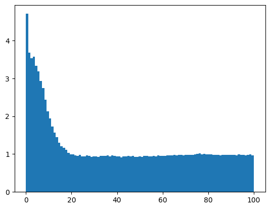
Relative pairwise distance distribution

A pairwise distance distribution relative to the expected distribution for a homogeneous sample (csr) reveals clustering effects.

bins = np.linspace(0, 100, 100)
hist_csr, bin_edges_csr = np.histogram(pd_csr_1.results.pair_distance, bins=bins, density=True)
hist_blob, bin_edges_blob = np.histogram(pd_blob_1.results.pair_distance, bins=bins, density=True)
bin_widths = np.diff(bin_edges_blob)
values = hist_blob / hist_csr

plt.bar(x=bin_edges_blob[:-1], height=values, align="edge", width=bin_widths, label="blob_1");