Tutorial about tracking LocData objects

Tracking refers to link localizations that are close in space over multiple frames and collect those localizations in individual tracks. We here make use of the trackpy package through wrapper functions to deal with LocData objects.

%matplotlib inline

import numpy as np
import pandas as pd
import matplotlib.pyplot as plt

import locan as lc

lc.show_versions(system=False, dependencies=False, verbose=False)

Locan:
   version: 0.22.0.dev32+g4bfc3ab8b

Python:
   version: 3.11.14

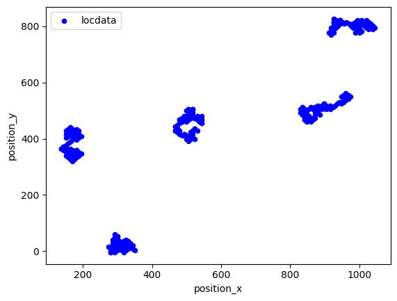
Synthetic data

A random dataset is created.

dat = lc.simulate_tracks(n_walks=5, n_steps=100, ranges=((0,1000),(0,1000)),
                      diffusion_constant=1, seed=1)

dat.print_meta()

Jupyter environment detected. Enabling Open3D WebVisualizer.
[Open3D INFO] WebRTC GUI backend enabled.
[Open3D INFO] WebRTCWindowSystem: HTTP handshake server disabled.

identifier: "1"
source: SIMULATION
state: RAW
history {
  name: "simulate_tracks"
  parameter: "{\'n_walks\': 5, \'n_steps\': 100, \'ranges\': ((0, 1000), (0, 1000)), \'diffusion_constant\': 1, \'time_step\': 10, \'seed\': 1}"
}
element_count: 500
frame_count: 100
creation_time {
  2026-04-30T08:38:41.872536Z
}

dat.data.head()

	position_x	position_y	frame
0	518.146180	429.651004	0
1	524.470735	435.975560	1
2	530.795291	429.651004	2
3	524.470735	435.975560	3
4	518.146180	429.651004	4

fig, ax = plt.subplots(nrows=1, ncols=1)
dat.data.plot.scatter(x='position_x', y='position_y', ax=ax, color='Blue', label='locdata')
plt.show()

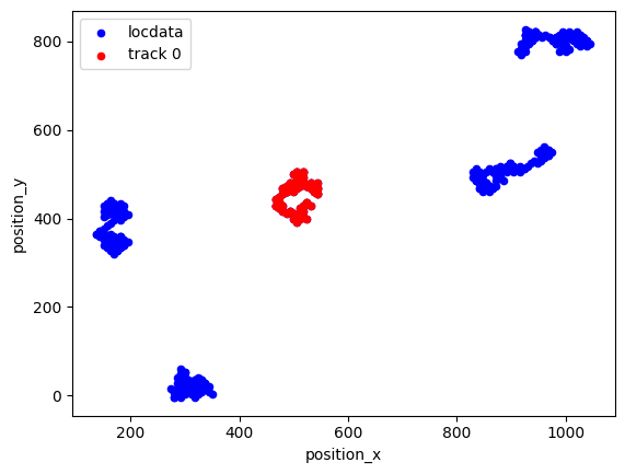
Track locdata

The track function collects tracks in a new locdata object.

tracks, track_numbers = lc.track(dat, search_range=500)

Frame 99: 5 trajectories present.

tracks.print_summary()

identifier: "7"
comment: ""
source: DESIGN
state: RAW
element_count: 5
frame_count: 1
creation_time {
  2026-04-30T08:38:42.201640Z
}

tracks.data

	localization_count	position_x	uncertainty_x	position_y	uncertainty_y	frame	region_measure_bb	localization_density_bb	subregion_measure_bb
0	100	505.497069	2.098581	456.720101	3.047211	0	8640.0	0.011574	379.473319
1	100	972.599640	3.900272	805.187177	1.217117	0	7560.0	0.013228	379.473319
2	100	169.710816	1.293090	381.371093	3.679042	0	6840.0	0.014620	354.175098
3	100	882.368107	4.321878	504.562854	2.382224	0	14720.0	0.006793	493.315315
4	100	307.151281	1.787996	19.463682	1.378273	0	4800.0	0.020833	278.280434

tracks.references[0].data.head()

	position_x	position_y	frame
0	518.146180	429.651004	0
1	524.470735	435.975560	1
2	530.795291	429.651004	2
3	524.470735	435.975560	3
4	518.146180	429.651004	4

fig, ax = plt.subplots(nrows=1, ncols=1)
dat.data.plot.scatter(x='position_x', y='position_y', ax=ax, color='Blue', label='locdata')
tracks.references[0].data.plot.scatter(x='position_x', y='position_y', ax=ax, color='Red', label='track 0')
plt.show()

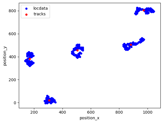
fig, ax = plt.subplots(nrows=1, ncols=1)
dat.data.plot.scatter(x='position_x', y='position_y', ax=ax, color='Blue', label='locdata')
tracks.data.plot.scatter(x='position_x', y='position_y', ax=ax, color='Red', label='tracks')
plt.show()

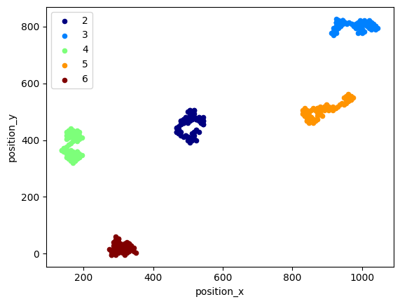
To show individual tracks make use of the reference attribute.

fig, ax = plt.subplots(nrows=1, ncols=1)

jet= plt.get_cmap('jet')
colors = iter(jet(np.linspace(0, 1, len(tracks))))

for ref in tracks.references:
    c=next(colors)
    ref.data.plot.scatter(x='position_x', y='position_y', ax=ax, color=(c,), label=ref.meta.identifier)

plt.show()

Alternatively to a new locdata object, a pandas DataFrame can be generated using the link_locdata method.

links = lc.link_locdata(dat, search_range=10)

Frame 99: 5 trajectories present.

links.head()

0      0
100    1
200    2
300    3
400    4
Name: track, dtype: int64

Use the following to add particle column to original locdata dataset.

dat.data.loc[links.index,'track']=links

dat.data.head()

	position_x	position_y	frame	track
0	518.146180	429.651004	0	0.0
1	524.470735	435.975560	1	0.0
2	530.795291	429.651004	2	0.0
3	524.470735	435.975560	3	0.0
4	518.146180	429.651004	4	0.0

Track using trackpy with locdata.data as input

For a detailed tracking analysis you might want to use trackpy functions with the pandas DataFrame carrying localization data as input. The following examples will igve a short illustration of using trackpy functions.

import trackpy as tp

t = tp.link_df(dat.data, search_range=100, memory=1, pos_columns=['position_x', 'position_y'], t_column='frame')

t.head(10)

Frame 99: 5 trajectories present.

	position_x	position_y	frame	track	particle
0	518.146180	429.651004	0	0.0	0
100	944.139141	821.378039	0	1.0	1
200	150.484168	402.874581	0	2.0	2
300	954.974002	543.269132	0	3.0	3
400	318.156007	33.883669	0	4.0	4
301	961.298558	549.593688	1	3.0	3
101	937.814586	815.053483	1	1.0	1
201	156.808723	409.199136	1	2.0	2
401	324.480563	27.559113	1	4.0	4
1	524.470735	435.975560	1	0.0	0

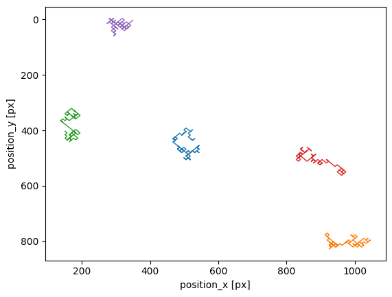
plt.figure()
tp.plot_traj(t, pos_columns=['position_x', 'position_y'], t_column='frame');

filter

t.head()

	position_x	position_y	frame	track	particle
0	518.146180	429.651004	0	0.0	0
100	944.139141	821.378039	0	1.0	1
200	150.484168	402.874581	0	2.0	2
300	954.974002	543.269132	0	3.0	3
400	318.156007	33.883669	0	4.0	4

t1 = tp.filter_stubs(t, 10).reset_index(drop=True)
len(t1)

500

plt.figure()
tp.plot_traj(t1, pos_columns=['position_x', 'position_y']);

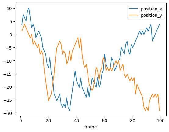
drift

d = tp.compute_drift(t1, pos_columns=['position_x', 'position_y'])

d.plot()
plt.show()

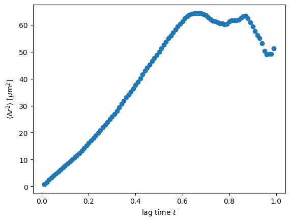
Mean square displacement (msd)

em = tp.emsd(t1,0.1, 100, pos_columns=['position_x', 'position_y']) # microns per pixel = 100/285., frames per second = 24

fig, ax = plt.subplots()
ax.plot(em.index, em, 'o')
#ax.set_xscale('log')
#ax.set_yscale('log')
ax.set(ylabel=r'$\langle \Delta r^2 \rangle$ [$\mu$m$^2$]',
       xlabel='lag time $t$')
#ax.set(ylim=(1e-2, 10));

[Text(0, 0.5, '$\\langle \\Delta r^2 \\rangle$ [$\\mu$m$^2$]'),
 Text(0.5, 0, 'lag time $t$')]