Tutorial about transforming LocData

Locan provides methods for transforming localization data sets into new LocData objects.

from pathlib import Path

%matplotlib inline

import numpy as np
import pandas as pd
import matplotlib.pyplot as plt
from mpl_toolkits.mplot3d import Axes3D

import locan as lc

lc.show_versions(system=False, dependencies=False, verbose=False)

Locan:
   version: 0.22.0.dev32+g4bfc3ab8b

Python:
   version: 3.11.14

# A path in which test data can be found:
TEST_DIR: Path = Path.cwd().parents[2] / "tests"
TEST_DIR

PosixPath('/home/docs/checkouts/readthedocs.org/user_builds/locan/checkouts/latest/tests')

Spatially randomize a structured set of localizations

Assume that localizations are somehow structured throughout a region. Often it is helpful to compare analysis results to a similar dataset in which localizations are homogeneously Poisson distributed. A LocData object with this kind of data can be provided by the randomize function.

rng = np.random.default_rng(seed=1)

locdata = lc.simulate_Thomas(parent_intensity=1e-5, region=((0, 1000), (0, 1000)), cluster_mu=100, cluster_std=10, seed=rng)
locdata.print_summary()

Jupyter environment detected. Enabling Open3D WebVisualizer.
[Open3D INFO] WebRTC GUI backend enabled.
[Open3D INFO] WebRTCWindowSystem: HTTP handshake server disabled.

identifier: "1"
comment: ""
source: SIMULATION
state: RAW
element_count: 705
frame_count: 0
creation_time {
  2026-04-30T08:38:46.629717Z
}

locdata_random = lc.randomize(locdata, hull_region='bb', seed=rng)

fig, ax = plt.subplots(nrows=1, ncols=2)
locdata.data.plot.scatter(x='position_x', y='position_y', ax=ax[0], color='Blue', label='locdata')
locdata_random.data.plot.scatter(x='position_x', y='position_y', ax=ax[1], color='Blue', label='locdata')
plt.tight_layout()
plt.show()

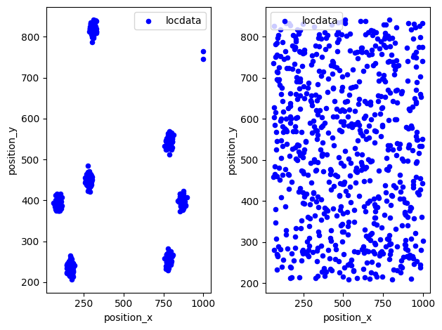
print('Area of bounding box for structured data: {:.0f}'.format(locdata.properties['region_measure_bb']))
print('Area of bounding box for randomized data: {:.0f}'.format(locdata_random.properties['region_measure_bb']))
print('Ratio: {:.4f}'.format(locdata_random.properties['region_measure_bb'] / locdata.properties['region_measure_bb']))

Area of bounding box for structured data: 595088
Area of bounding box for randomized data: 592451
Ratio: 0.9956

Regions other from bounding box can be specified as RoiRegion instance.

region = lc.ConvexHull(locdata.coordinates).region
locdata_random = lc.randomize(locdata, hull_region=region)

fig, ax = plt.subplots(nrows=1, ncols=2)
locdata.data.plot.scatter(x='position_x', y='position_y', ax=ax[0], color='Blue', label='locdata')
locdata_random.data.plot.scatter(x='position_x', y='position_y', ax=ax[1], color='Blue', label='locdata')
plt.tight_layout()
plt.show()

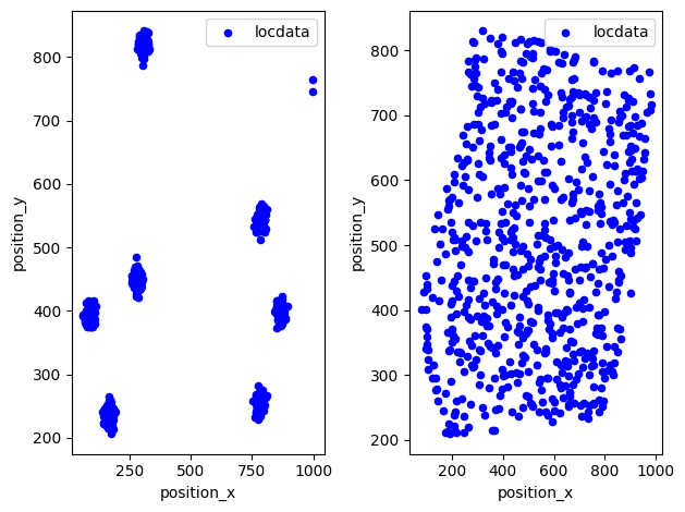
print('Area of bounding box for structured data: {:.0f}'.format(locdata.properties['region_measure_bb']))
print('Area of bounding box for randomized data: {:.0f}'.format(locdata_random.properties['region_measure_bb']))
print('Ratio: {:.4f}'.format(locdata_random.properties['region_measure_bb'] / locdata.properties['region_measure_bb']))

Area of bounding box for structured data: 595088
Area of bounding box for randomized data: 558742
Ratio: 0.9389

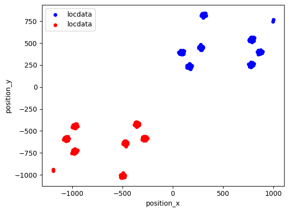
Apply an affine transformation to localization coordinates

A wrapper function provides affine transformations based on either numpy or open3d methods.

matrix = ((-1, 0), (0, -1))
offset = (10, 10)
pre_translation = (100, 100)

locdata_transformed = lc.transform_affine(locdata, matrix, offset, pre_translation, method='numpy')

fig, ax = plt.subplots()
locdata.data.plot.scatter(x='position_x', y='position_y',color='Blue', label='locdata', ax=ax)
locdata_transformed.data.plot.scatter(x='position_x', y='position_y', color='Red', label='locdata', ax=ax);

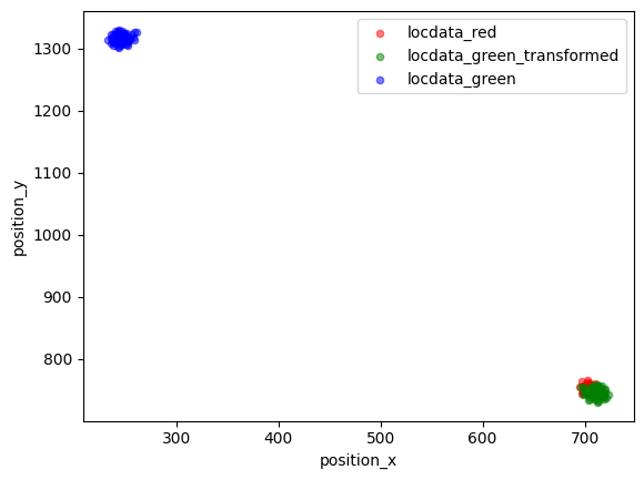
Apply a BunwarpJ transformation to localization coordinates

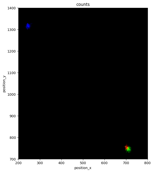
Often a transformation matrix was computed using ImageJ. The bunwarp function allows applying a transformation from the raw matrix of the ImageJ/Fiji plugin BunwarpJ. Here we show a very small region with a single fluorescent bead that is recorded on a red and a green dSTORM channel.

matrix_path = TEST_DIR / 'test_data/transform/BunwarpJ_transformation_raw_green.txt'
locdata_green = lc.load_asdf_file(path=TEST_DIR /
                                 'test_data/transform/rapidSTORM_beads_green.asdf')
locdata_red = lc.load_asdf_file(path=TEST_DIR /
                                 'test_data/transform/rapidSTORM_beads_red.asdf')

locdata_green_transformed = lc.bunwarp(locdata=locdata_green, matrix_path=matrix_path, pixel_size=(10, 10), flip=True)

fig, ax = plt.subplots()
locdata_red.data.plot.scatter(x='position_x', y='position_y',color='Red', label='locdata_red', alpha=0.5, ax=ax)
locdata_green_transformed.data.plot.scatter(x='position_x', y='position_y', color='Green', label='locdata_green_transformed', alpha=0.5, ax=ax)
locdata_green.data.plot.scatter(x='position_x', y='position_y',color='Blue', label='locdata_green', alpha=0.5, ax=ax);

fig, ax = plt.subplots(figsize=(10, 8))
lc. render_2d_rgb_mpl([locdata_red, locdata_green_transformed, locdata_green], bin_size=5, bin_range=((200, 800), (700, 1400)), rescale=lc.Trafo.EQUALIZE_0P3, ax=ax);