Tutorial about how to use a standard Analysis class
from pathlib import Path

%matplotlib inline

import matplotlib.pyplot as plt

import locan as lc
lc.show_versions(system=False, dependencies=False, verbose=False)
Locan:
   version: 0.22.0.dev32+g4bfc3ab8b

Python:
   version: 3.11.14
# A path in which test data can be found:
TEST_DIR: Path = Path.cwd().parents[2] / "tests"
TEST_DIR
PosixPath('/home/docs/checkouts/readthedocs.org/user_builds/locan/checkouts/latest/tests')
Load SMLM data file
Identify some data in the test_data directory and provide a path using pathlib.Path
path = TEST_DIR / 'test_data/npc_gp210.asdf'
print(path, '\n')
dat = lc.load_locdata(path=path, file_type=lc.FileType.ASDF)
/home/docs/checkouts/readthedocs.org/user_builds/locan/checkouts/latest/tests/test_data/npc_gp210.asdf
Jupyter environment detected. Enabling Open3D WebVisualizer.
[Open3D INFO] WebRTC GUI backend enabled.
[Open3D INFO] WebRTCWindowSystem: HTTP handshake server disabled.
print(dat.data.head(), '\n')
print('Summary:')
dat.print_summary()
print('Properties:')
print(dat.properties)
    position_x   position_y  frame     intensity  two_kernel_improvement  \
0  5631.709961  6555.850098     24  21800.699219                     0.0
1  5642.899902  6550.990234     25  23352.900391                     0.0
2  5610.319824  6546.819824     26   5007.509766                     0.0
3  5713.299805  6611.950195    141   6437.140137                     0.0
4  5699.750000  6627.390137    142  19998.300781                     0.0

   chi_square  local_background
0   1426930.0       1188.489990
1    983634.0       1135.199951
2    577707.0       1107.219971
3    616255.0       1118.430054
4    903412.0       1144.709961

Summary:
identifier: "5"
comment: ""
source: EXPERIMENT
state: MODIFIED
element_count: 202
frame_count: 202
file {
  type: ASDF
  path: "/home/docs/checkouts/readthedocs.org/user_builds/locan/checkouts/latest/tests/test_data/npc_gp210.asdf"
}
creation_time {
  2024-01-23T08:32:31.518779Z
}
modification_time {
  2024-01-23T08:32:31.518779Z
}

Properties:
{'localization_count': 202, 'position_x': np.float64(5623.488892810179), 'uncertainty_x': np.float64(3.9700846636030356), 'position_y': np.float64(6625.534602703435), 'uncertainty_y': np.float64(3.999303432482808), 'intensity': np.float32(3944778.0), 'local_background': np.float32(1131.3207), 'frame': np.int16(24), 'region_measure_bb': np.float32(47134.543), 'localization_density_bb': np.float32(0.004285604), 'subregion_measure_bb': np.float32(870.98047)}
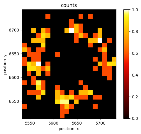
Visualization
For visualizing the data use one of the rendering methods.
lc.render_2d_mpl(dat, bin_size=10, rescale=lc.Trafo.EQUALIZE);
A simple analysis procedure: localization precision
Instantiation
Create an instance of the analysis class. By doing this you set all parameters in the parameter attribute. To start the actual computation you have to call instance.compute().
lp = lc.LocalizationPrecision(radius=50)
Each analysis class provides some attributes and methods for the most common interactions with the computed results.
attributes = [x for x in dir(lp) if not x.startswith('_')]
attributes
['compute',
 'count',
 'distribution_statistics',
 'fit_distributions',
 'hist',
 'meta',
 'parameter',
 'plot',
 'report',
 'results']
The results attribute
A standard analysis class has an attribute results to hold the most fundamental results as number, numpy array or pandas series or dataframe.
lp.compute(dat)
print('type of lpf.results: ', type(lp.results), '\n')
print(lp.results.head())
Processed frames:: 0%| | 0/24884 [00:00<?, ?it/s]
Processed frames:: 0%| | 1/24884 [00:00<56:23, 7.36it/s]
Processed frames:: 16%|█▌ | 3906/24884 [00:00<00:01, 19663.80it/s]
Processed frames:: 29%|██▉ | 7266/24884 [00:00<00:00, 25235.78it/s]
Processed frames:: 69%|██████▉ | 17286/24884 [00:00<00:00, 52753.34it/s]
Processed frames:: 100%|██████████| 24884/24884 [00:00<00:00, 50701.69it/s]
type of lpf.results:  <class 'pandas.core.frame.DataFrame'>

   position_delta_x  position_delta_y  position_distance  original_index  \
0        -11.189941          4.859863          12.199716               0
1         32.580078          4.170410          32.845909               1
2         13.549805        -15.439941          20.542370               3
3          4.669922          3.010254           5.556060               4
4         20.469727         14.750000          25.230383               6

   frame
0     24
1     25
2    141
3    142
4    239
Results can be saved by specifying a path
from pathlib import Path
temp_directory = Path('.') / 'temp'
temp_directory.mkdir(parents=True, exist_ok=True)

path = temp_directory / 'results.txt'
path
PosixPath('temp/results.txt')
and saving the data using numpy or pandas routines
lp.results.to_csv(path, sep='\t')
Delete the file and empty directory
path.unlink()
temp_directory.rmdir()
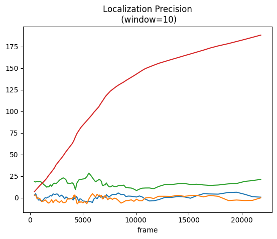
A simple standardized plot
Most likely the results should be inspected by looking at a typical plot. In this case the plot shows results smoothed by a running average according to the specified window.
lp.plot(window=10);
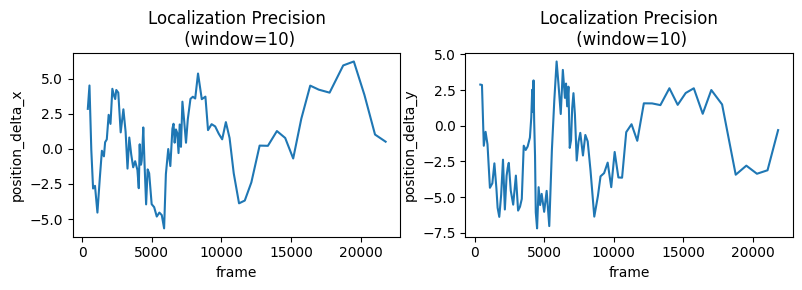
For more advanced plotting schemes use the matplotlip framework.
fig, ax = plt.subplots(nrows=1, ncols=2, figsize=(8,3))
lp.plot(ax=ax[0], window=10, loc_property='position_delta_x')
lp.plot(ax=ax[1], window=10, loc_property='position_delta_y')
plt.tight_layout()
plt.show()
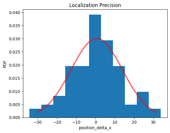
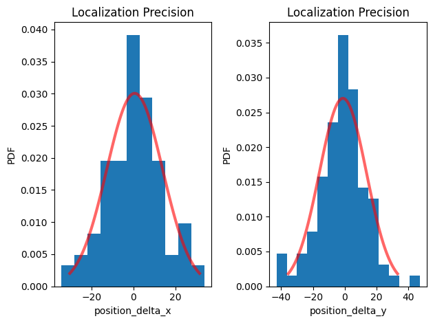
A simple standardized histogram
Quite often the results are best presented as a histogram. The histogram for the distances per default includes a fit to a distribution expected for normal distributed localizations. Sigma is the localization precision.
The histogram per default provides automatic bins and is normalized to show a probability density function.
lp.hist(loc_property='position_delta_x');
Alternatively the position deltas can be histogrammed.
fig, ax = plt.subplots(nrows=1, ncols=2)
lp.hist(ax=ax[0], loc_property='position_delta_x')
lp.hist(ax=ax[1], loc_property='position_delta_y')
plt.tight_layout()
plt.show()
Secondary results
Secondary results are e.g. fit parameter derived from analyzing the distribution of results values. Secondary results are different for each analysis routine. They are included as additional attributes.
Localization precision can e.g. be derived from fitting the position distances to an appropriate distribution and estimating the sigma parameter.
lp.distribution_statistics.parameter_dict()
{'position_delta_x_loc': np.float32(0.6029139),
 'position_delta_x_scale': np.float32(13.2682),
 'position_delta_y_loc': np.float32(-1.227687),
 'position_delta_y_scale': np.float32(14.76087),
 'position_distance_sigma': np.float64(14.067675781250028),
 'position_distance_loc': 0,
 'position_distance_scale': 1}
print('position_distance_sigma: ', lp.distribution_statistics.parameter_dict()['position_distance_sigma'])
position_distance_sigma: 14.067675781250028
Metadata
Each analysis class is supplied with meta data. The main purpose is to (i) capture methods and parameters that were supplied in each instantiation and (ii) provide information on the dataset on which the particular analysis was carried out. Metadata is structured using protocol buffers.
lp.meta
identifier: "1"
method {
  name: "LocalizationPrecision"
  parameter: "{\'radius\': 50}"
}
creation_time {
  seconds: 1777538078
  nanos: 626496000
}
You can add some user-defined key-value pairs:
lp.meta.map['some key'] = 'some value'
lp.meta.map
{'some key': 'some value'}
Metadata can be used to rerun the analysis with the same parameter.
lp.meta.method.name
'LocalizationPrecision'
lp.meta.method.parameter
"{'radius': 50}"
import ast
import locan.analysis
params = ast.literal_eval(lp.meta.method.parameter)
print(params)
lp_2 = getattr(locan.analysis, lp.meta.method.name)(**params)
lp_2.compute(dat)
lp_2.results.head()
{'radius': 50}
Processed frames:: 0%| | 0/24884 [00:00<?, ?it/s]
Processed frames:: 16%|█▌ | 3905/24884 [00:00<00:00, 38163.35it/s]
Processed frames:: 31%|███ | 7722/24884 [00:00<00:00, 36637.62it/s]
Processed frames:: 70%|██████▉ | 17361/24884 [00:00<00:00, 62934.63it/s]
Processed frames:: 100%|██████████| 24884/24884 [00:00<00:00, 69930.64it/s]
| position_delta_x | position_delta_y | position_distance | original_index | frame | |
|---|---|---|---|---|---|
| 0 | -11.189941 | 4.859863 | 12.199716 | 0 | 24 |
| 1 | 32.580078 | 4.170410 | 32.845909 | 1 | 25 |
| 2 | 13.549805 | -15.439941 | 20.542370 | 3 | 141 |
| 3 | 4.669922 | 3.010254 | 5.556060 | 4 | 142 |
| 4 | 20.469727 | 14.750000 | 25.230383 | 6 | 239 |