Tutorial about Ripley’s k function

from pathlib import Path

%matplotlib inline

import numpy as np
import matplotlib.pyplot as plt

import locan as lc

lc.show_versions(system=False, dependencies=False, verbose=False)

Locan:
   version: 0.22.0.dev32+g4bfc3ab8b

Python:
   version: 3.11.14

Synthetic data

We simulate localization data that is homogeneously Poisson distributed (also described as complete spatial randomness, csr).

rng = np.random.default_rng(seed=1)

locdata_csr = lc.simulate_Poisson(intensity=1e-3, region=((0,1000), (0,1000)), seed=rng)

print('Data head:')
print(locdata_csr.data.head(), '\n')
print('Summary:')
locdata_csr.print_summary()
print('Properties:')
print(locdata_csr.properties)

Jupyter environment detected. Enabling Open3D WebVisualizer.
[Open3D INFO] WebRTC GUI backend enabled.
[Open3D INFO] WebRTCWindowSystem: HTTP handshake server disabled.

Data head:
   position_x  position_y
0  144.159613  948.649447
1  311.831452  423.326449
2  827.702594  409.199136
3  549.593688   27.559113
4  753.513109  538.143313 

Summary:
identifier: "1"
comment: ""
source: SIMULATION
state: RAW
element_count: 1001
frame_count: 0
creation_time {
  2026-04-30T08:33:31.799315Z
}

Properties:
{'localization_count': 1001, 'position_x': np.float64(497.1480704304259), 'uncertainty_x': np.float64(8.846806436903796), 'position_y': np.float64(503.49401443075675), 'uncertainty_y': np.float64(9.309630174812341), 'region_measure_bb': np.float64(997049.9168748705), 'localization_density_bb': np.float64(0.001003961770677952), 'subregion_measure_bb': np.float64(3994.0982202393607), 'region_measure': np.int64(1000000), 'localization_density': np.float64(0.001001), 'subregion_measure': np.int64(4000)}

We also simulate data that follows a Neyman-Scott distribution (blobs):

locdata_blob = lc.simulate_Thomas(parent_intensity=1e-4, region=((0, 1000), (0, 1000)), cluster_mu=100, cluster_std=5, seed=rng)

print('Data head:')
print(locdata_blob.data.head(), '\n')
print('Summary:')
locdata_blob.print_summary()
print('Properties:')
print(locdata_blob.properties)

Data head:
   position_x  position_y  cluster_label
0    0.661558   79.743448            106
1  311.655699   92.446213             17
2  874.374807  274.998314             27
3  136.056776  315.663828             20
4  396.397559  721.160904             34 

Summary:
identifier: "2"
comment: ""
source: SIMULATION
state: RAW
element_count: 10630
frame_count: 0
creation_time {
  2026-04-30T08:33:31.828904Z
}

Properties:
{'localization_count': 10630, 'position_x': np.float64(497.79301818419225), 'uncertainty_x': np.float64(2.876128036271366), 'position_y': np.float64(500.16721842421566), 'uncertainty_y': np.float64(2.8846099186586316), 'region_measure_bb': np.float64(999157.130817876), 'localization_density_bb': np.float64(0.010638967257631084), 'subregion_measure_bb': np.float64(3998.3141398027747), 'region_measure': np.int64(1000000), 'localization_density': np.float64(0.01063), 'subregion_measure': np.int64(4000)}

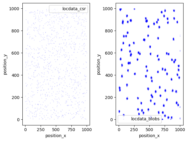
Scatter plot

fig, ax = plt.subplots(nrows=1, ncols=2)
locdata_csr.data.plot.scatter(x='position_x', y='position_y', ax=ax[0], color='Blue', s=1, alpha=0.1, label='locdata_csr')
locdata_blob.data.plot.scatter(x='position_x', y='position_y', ax=ax[1], color='Blue', s=1, alpha=0.1, label='locdata_blobs')
plt.tight_layout()
plt.show()

Analyze Ripley’s h function

We have a look at the Ripley’s h function from all localizations in locdata.

The analysis class Ripley_h_function provides numerical results, and a plot of results versus radii.

rhf_csr = lc.RipleysHFunction(radii=np.linspace(0, 200, 50))
rhf_csr.compute(locdata_csr)
rhf_csr.results.head()

	Ripley_h_data
radius
0.000000	0.000000
4.081633	0.279930
8.163265	-0.240094
12.244898	-0.194560
16.326531	-0.301127

rhf_blob = lc.RipleysHFunction(radii=np.linspace(0, 200, 50))
rhf_blob.compute(locdata_blob)
rhf_blob.results.head()

	Ripley_h_data
radius
0.000000	0.000000
4.081633	17.927448
8.163265	31.067851
12.244898	37.498780
16.326531	38.678837

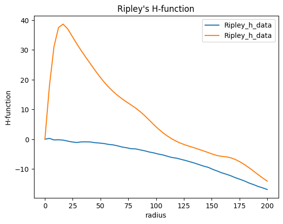
The plot reflects the amount of clustering. For homogeneous distributed data it decreases towards negative values since edge effects are not taken into account.

rhf_csr.plot()
rhf_blob.plot();

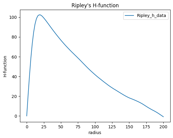
The maximum of the computed H-function is provided by the attribute.

rhf_blob.Ripley_h_maximum

	radius	Ripley_h_maximum
Ripley_h_data	16.326531	38.678837

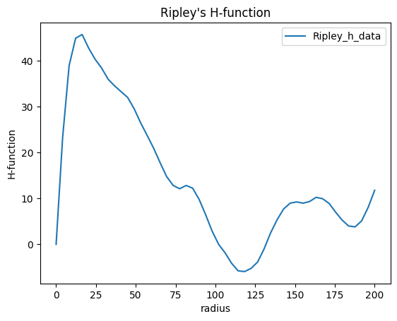
Estimate Ripley’s h function

We can speed up the computation of an estimated Ripley’s k function by providing a subset of the original localizations as test points.

We first take a random subset of the original localizations as test data. Here we provide 10 shuffeled data sets.

from locan.process.filter import random_subset
subsets = [lc.random_subset(locdata_blob, n_points=5, seed=rng) for i in range(10)]

We then compute the estimated Ripley’s h function’

rhf_estimate = lc.RipleysHFunction(radii=np.linspace(0, 200, 50)).compute(locdata_blob, other_locdata=subsets[0])

rhf_estimate.plot();

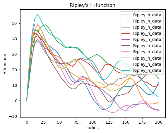
We can do the same for all subsets

rhf_estimates = [lc.RipleysHFunction(radii=np.linspace(0, 200, 50)).compute(locdata_blob, other_locdata=subset) for subset in subsets]

fig, ax = plt.subplots(nrows=1, ncols=1)
for estimate in rhf_estimates:
    estimate.plot(ax=ax)
plt.show()

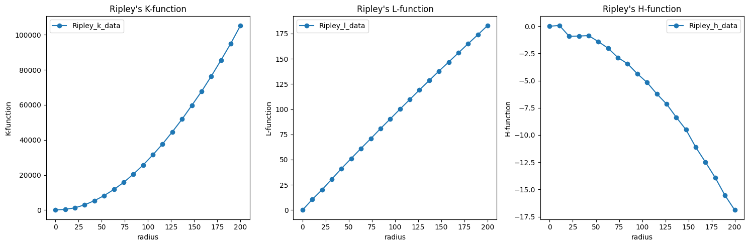
Compute Ripley’s k, l and h function

We can compute Ripley’s k, l and h function

rkf_csr = lc.RipleysKFunction(radii=np.linspace(0, 200, 20)).compute(locdata_csr)
rlf_csr = lc.RipleysLFunction(radii=np.linspace(0, 200, 20)).compute(locdata_csr)
rhf_csr = lc.RipleysHFunction(radii=np.linspace(0, 200, 20)).compute(locdata_csr)

fig, axes = plt.subplots(nrows=1, ncols=3, figsize=(15, 5))
for estimate, ax in zip([rkf_csr, rlf_csr, rhf_csr], axes.ravel()):
    estimate.plot(marker='o', ax=ax)
plt.tight_layout()
plt.show()

Estimate Ripley’s h function for 3D data

dat_blob_3D = lc.simulate_Thomas(parent_intensity=1e-7, region=((0, 1000), (0, 1000), (0, 1000)), cluster_mu=100, cluster_std=5, seed=rng)
dat_blob_3D.print_summary()

identifier: "23"
comment: ""
source: SIMULATION
state: RAW
element_count: 12403
frame_count: 0
creation_time {
  2026-04-30T08:33:37.722946Z
}

sub = lc.random_subset(dat_blob_3D, n_points=1000, seed=rng)

rhf_3D = lc.RipleysHFunction(radii=np.linspace(0, 200, 100)).compute(dat_blob_3D, other_locdata=sub)

rhf_3D.plot();