Tutorial about coordinate-based colocalization
Coordinate-based colocalization of two selections is computed as introduced by Malkusch et al. (1). A local density of locdata A is compared with the local density of locdata B within a varying radius for each localization in selection A. Local densities at various radii are compared by Spearman-rank-correlation and weighted by an exponential factor including the Euclidean distance to the nearest neighbor for each localization. The colocalization coefficient can take a value between -1 and 1 with -1 indicating anti-correlation (i.e. nearby localizations of selection B), 0 no colocalization, 1 strong colocalization.
The colocalization coefficient is provided as property for each localization within the corresponding dataset. The property key refers to colocalizing locdata A with locdata B.
from pathlib import Path

%matplotlib inline

import numpy as np
import pandas as pd
import matplotlib.pyplot as plt
import matplotlib.colors as colors

import locan as lc
lc.show_versions(system=False, dependencies=False, verbose=False)
Locan:
   version: 0.22.0.dev32+g4bfc3ab8b

Python:
   version: 3.11.14
Synthetic data
Provide synthetic data made of clustered localizations that are normal distributed around their center positions.
rng = np.random.default_rng(seed=1)
def set_centers(n_centers_1d=3, feature_range = (0, 1000)):
    dist = (feature_range[1] - feature_range[0])/(n_centers_1d + 1)
    centers = np.mgrid[feature_range[0] + dist : feature_range[1] : dist, feature_range[0] + dist : feature_range[1] : dist].reshape(2, -1).T
    return centers
n_centers_1d = 3
feature_range = (0, 1000)
centers = set_centers(n_centers_1d, feature_range)
offspring = rng.normal(loc=0, scale=20, size=(len(centers), 100, 2))
locdata = lc.simulate_cluster(centers=centers, region=[feature_range] * 2, offspring=offspring, clip=True, shuffle=True, seed=rng)

locdata.print_summary()
Jupyter environment detected. Enabling Open3D WebVisualizer.
[Open3D INFO] WebRTC GUI backend enabled.
[Open3D INFO] WebRTCWindowSystem: HTTP handshake server disabled.
identifier: "1"
comment: ""
source: SIMULATION
state: RAW
element_count: 900
frame_count: 0
creation_time {
  2026-04-30T08:33:41.792546Z
}
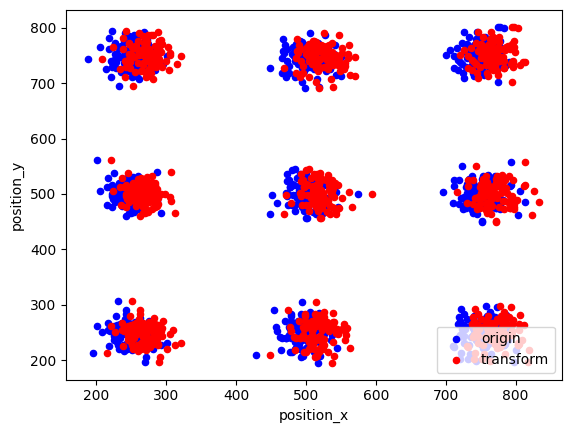
A second dataset is provided by shifting the first dataset by an offset.
locdata_trans = lc.transform_affine(locdata, offset=(20,0))
locdata_trans.print_summary()
identifier: "2"
comment: ""
source: SIMULATION
state: MODIFIED
element_count: 900
frame_count: 0
creation_time {
  2026-04-30T08:33:41.792546Z
}
modification_time {
  2026-04-30T08:33:41.882659Z
}
fig, ax = plt.subplots(nrows=1, ncols=1)
locdata.data.plot.scatter(x='position_x', y='position_y', ax=ax, color='Blue', label='origin')
locdata_trans.data.plot.scatter(x='position_x', y='position_y', ax=ax, color='Red', label='transform')
plt.show()
CBC computation
cbc = lc.CoordinateBasedColocalization(radius=100, n_steps=10).compute(locdata=locdata, other_locdata=locdata_trans)
cbc.results.head()
| colocalization_cbc_2 | |
|---|---|
| 0 | 0.382530 |
| 1 | 0.280571 |
| 2 | 0.036730 |
| 3 | 0.152874 |
| 4 | 0.385790 |
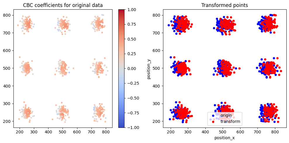
Results
points = locdata.coordinates
color = cbc.results['colocalization_cbc_2'].values

fig, axes = plt.subplots(nrows=1, ncols=2, figsize=(10, 5))
cax = axes[0].scatter(x=points[:,0], y=points[:,1], marker='.', c=color, cmap='coolwarm', norm= colors.Normalize(-1., 1.), label='points')
axes[0].set_title('CBC coefficients for original data')

# axes[1].scatter(x=points[:,0], y=points[:,1], marker='.', color='Blue', label='points')
# axes[1].scatter(x=points_trans[:,0], y=points_trans[:,1], marker='o', color='Red', label='transformed points')
locdata.data.plot.scatter(x='position_x', y='position_y', ax=axes[1], color='Blue', label='origin')
locdata_trans.data.plot.scatter(x='position_x', y='position_y', ax=axes[1], color='Red', label='transform')
axes[1].set_title('Transformed points')
plt.colorbar(cax, ax=axes[0])
plt.tight_layout()
plt.show()
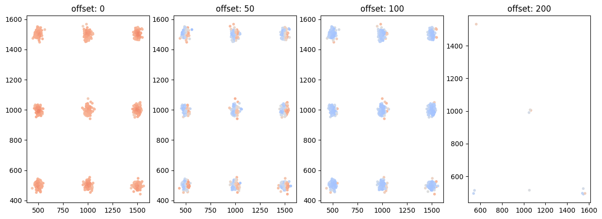
CBC for various shifts
n_centers_1d = 3
feature_range = (0, 2000)
centers = set_centers(n_centers_1d, feature_range)
offspring = rng.normal(loc=0, scale=20, size=(len(centers), 100, 2))
locdata = lc.simulate_cluster(centers=centers, region=[feature_range] * 2, offspring=offspring, clip=True, shuffle=True, seed=rng)

locdata.print_summary()
identifier: "3"
comment: ""
source: SIMULATION
state: RAW
element_count: 900
frame_count: 0
creation_time {
  2026-04-30T08:33:43.437022Z
}
offsets = [0, 50, 100, 200]
locdata_trans_list = [lc.transform_affine(locdata, offset=(offset, 0)) for offset in offsets]
cbc_list = [lc.CoordinateBasedColocalization(radius=100, n_steps=10).compute(locdata=locdata, other_locdata=other_locdata) for other_locdata in locdata_trans_list]
points = locdata.coordinates
n_rows = 1
n_cols = 4

fig = plt.figure(figsize=(15, 5))
for n, (cbc, offset) in enumerate(zip(cbc_list, offsets)):
    ax = fig.add_subplot(n_rows, n_cols, n+1)
    color = cbc.results.iloc[:, 0].values
    ax.scatter(x=points[:,0], y=points[:,1], marker='.', c=color, cmap='coolwarm', norm=colors.Normalize(-1., 1.))
    ax.set_title(f'offset: {offset}')
plt.show()
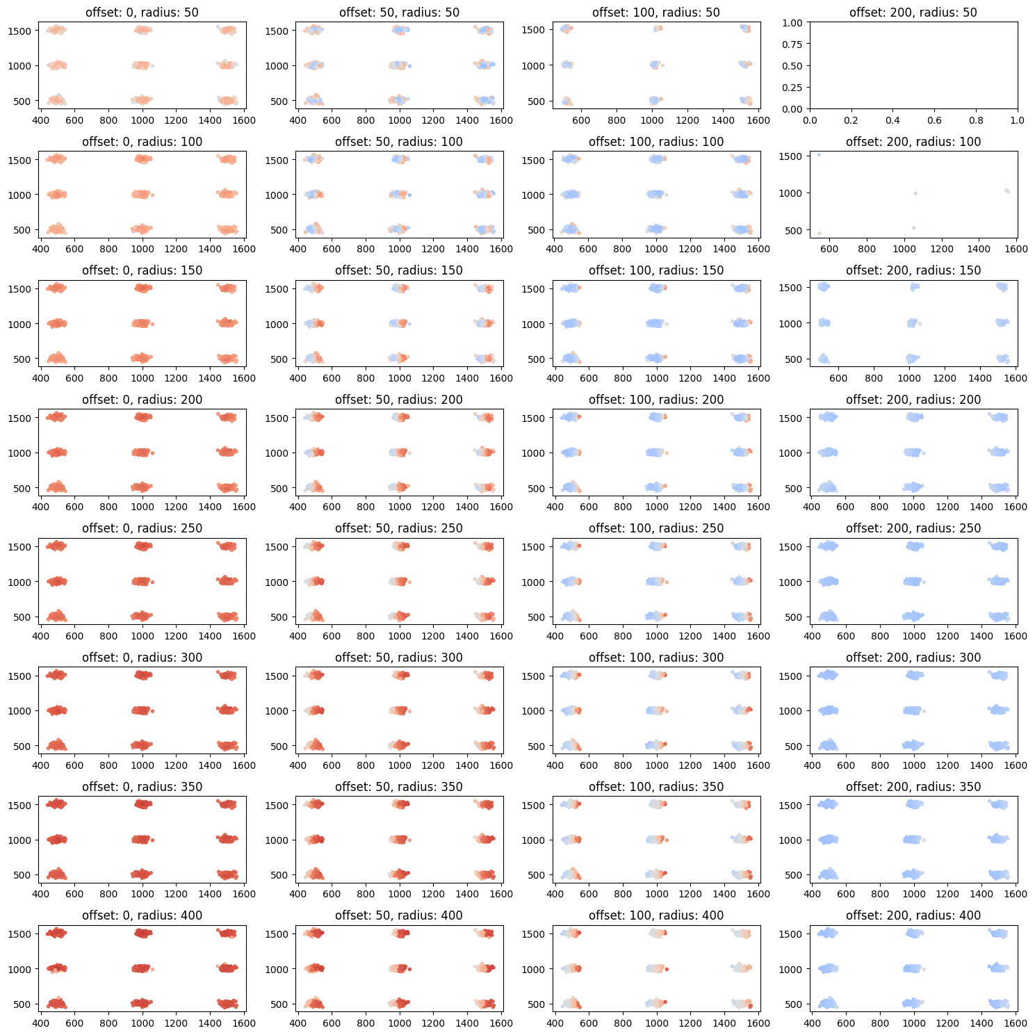
CBC on various length scales (for small cluster)
n_centers_1d = 3
feature_range = (0, 2000)
centers = set_centers(n_centers_1d, feature_range)
offspring = rng.normal(loc=0, scale=20, size=(len(centers), 100, 2))
locdata = lc.simulate_cluster(centers=centers, region=[feature_range] * 2, offspring=offspring, clip=True, shuffle=True, seed=rng)
offsets = [0, 50, 100, 200]
locdata_trans_list = [lc.transform_affine(locdata, offset=(offset,0)) for offset in offsets]
radii = [50, 100, 150, 200, 250, 300, 350, 400]
cbc_list = [lc.CoordinateBasedColocalization(radius=radius, n_steps=10).compute(locdata=locdata, other_locdata=other_locdata) for radius in radii
            for other_locdata in locdata_trans_list
           ]
points = locdata.coordinates
params = [(radius, offset) for radius in radii for offset in offsets]

n_rows = len(radii)
n_cols = len(offsets)

fig = plt.figure(figsize=(15, 15))
for n, (cbc, (radius, offset)) in enumerate(zip(cbc_list, params)):
    ax = fig.add_subplot(n_rows, n_cols, n+1)
    color = cbc.results.iloc[:, 0].values
    if not all(np.isnan(color)):
        ax.scatter(x=points[:,0], y=points[:,1], marker='.', c=color, cmap='coolwarm', norm=colors.Normalize(-1., 1.))
    ax.set_title(f'offset: {offset}, radius: {radius}')
plt.tight_layout()
plt.show()
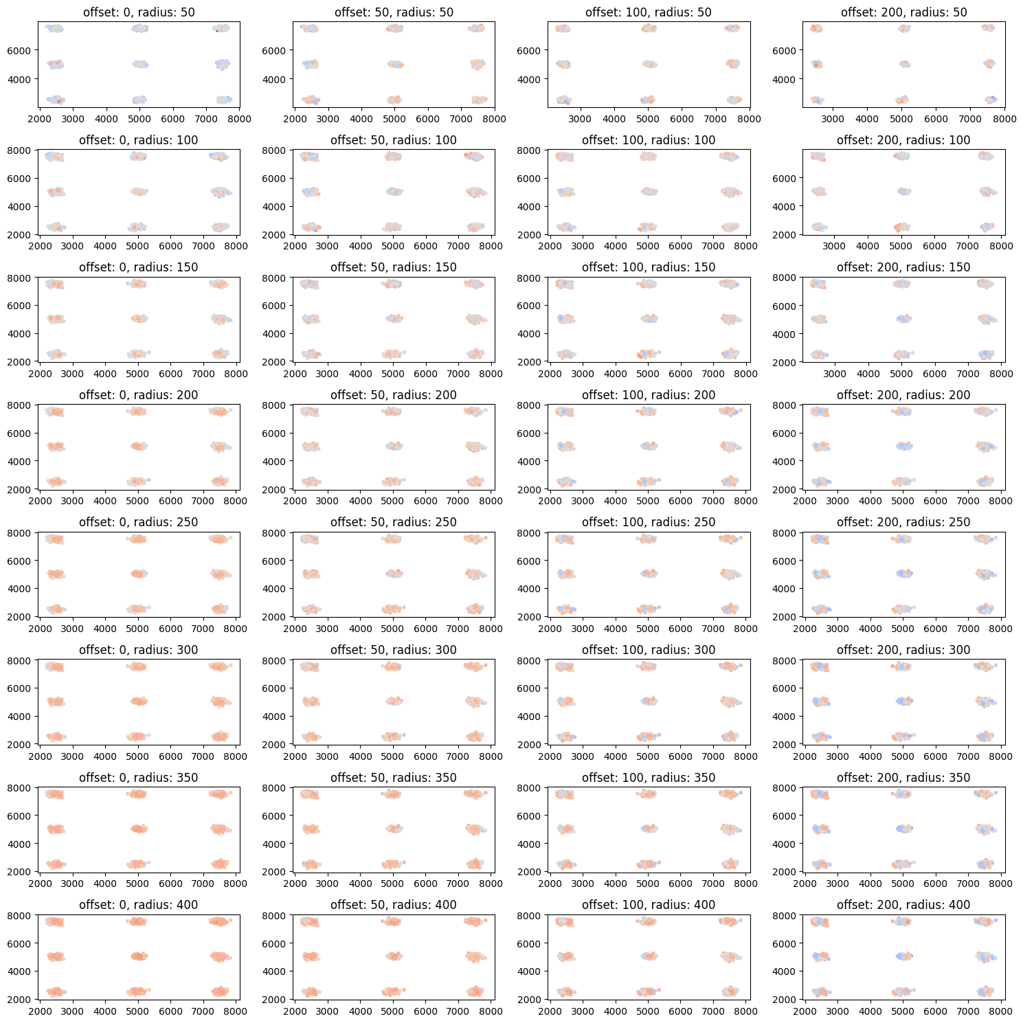
CBC on various length scales (for larger cluster)
n_centers_1d = 3
feature_range = (0, 10_000)
centers = set_centers(n_centers_1d, feature_range)
offspring = rng.normal(loc=0, scale=100, size=(len(centers), 100, 2))
locdata = lc.simulate_cluster(centers=centers, region=[feature_range] * 2, offspring=offspring, clip=True, shuffle=True, seed=rng)
offsets = [0, 50, 100, 200]
locdata_trans_list = [lc.transform_affine(locdata, offset=(offset,0)) for offset in offsets]
radii = [50, 100, 150, 200, 250, 300, 350, 400]
cbc_list = [lc.CoordinateBasedColocalization(radius=radius, n_steps=10).compute(locdata=locdata, other_locdata=other_locdata) for radius in radii
            for other_locdata in locdata_trans_list
           ]
points = locdata.coordinates
params = [(radius, offset) for radius in radii for offset in offsets]

n_rows = len(radii)
n_cols = len(offsets)

fig = plt.figure(figsize=(15, 15))
for n, (cbc, (radius, offset)) in enumerate(zip(cbc_list, params)):
    ax = fig.add_subplot(n_rows, n_cols, n+1)
    color = cbc.results.iloc[:, 0].values
    ax.scatter(x=points[:,0], y=points[:,1], marker='.', c=color, cmap='coolwarm', norm=colors.Normalize(-1., 1.))
    ax.set_title(f'offset: {offset}, radius: {radius}')
plt.tight_layout()
plt.show()