Tutorial about setting up an analysis pipeline and batch processing#

Quite often you experiment with various analysis routines and appropriate parameters and come up with an analysis pipeline. A pipeline procedure then is a script defining analysis steps for a single locdata object (or a single group of corresponding locdatas as for instance used in 2-color measurements).

The Pipeline class can be used to combine the pipeline code, metadata and analysis results in a single pickleable object (meaning it can be serialized by the python pickle module).

This pipeline might then be applied to a number of similar datasets. A batch process is such a procedure for running a pipeline over multiple locdata objects and collecting and combing results.

from pathlib import Path

%matplotlib inline

import matplotlib.pyplot as plt

import locan as lc

lc.show_versions(system=False, dependencies=False, verbose=False)

Locan:
   version: 0.20.0.dev41+g755b969

Python:
   version: 3.11.6

Apply a pipeline of different analysis routines#

Load rapidSTORM data file#

path = lc.ROOT_DIR / 'tests/test_data/npc_gp210.asdf'
print(path, '\n')
dat = lc.load_locdata(path=path, file_type=lc.FileType.ASDF)

/home/docs/checkouts/readthedocs.org/user_builds/locan/envs/latest/lib/python3.11/site-packages/locan/tests/test_data/npc_gp210.asdf 

Jupyter environment detected. Enabling Open3D WebVisualizer.
[Open3D INFO] WebRTC GUI backend enabled.
[Open3D INFO] WebRTCWindowSystem: HTTP handshake server disabled.

dat.properties

{'localization_count': 202,
 'position_x': 5623.488892810179,
 'uncertainty_x': 3.9700846636030356,
 'position_y': 6625.534602703435,
 'uncertainty_y': 3.999303432482808,
 'intensity': 3944778.0,
 'local_background': 1131.3207,
 'frame': 24,
 'region_measure_bb': 47134.543,
 'localization_density_bb': 0.00428560429946091,
 'subregion_measure_bb': 870.98046875}

Set up an analysis procedure#

First define the analysis procedure (pipeline) in form of a computation function. Make sure the first parameter is the self refering to the Pipeline object. Add arbitrary keyword arguments thereafter. When finishing with return self the compute method can easily be called with instantiation.

def computation(self, locdata, n_localizations_min=4):
    
    # import required modules
    from locan.analysis import LocalizationPrecision
    
    # prologue
    self.file_indicator = locdata.meta.file.path
    self.locdata = locdata
    
    # check requirements
    if len(locdata)<=n_localizations_min:
        return None
    
    # compute localization precision
    self.lp = LocalizationPrecision().compute(self.locdata)
    
    return self

Run the analysis procedure#

Instantiate a Pipeline object and run compute():

pipe = lc.Pipeline(computation=computation, locdata=dat, n_localizations_min=4).compute()
pipe.meta

Processed frames::   0%|          | 0/24884 [00:00<?, ?it/s]

Processed frames::   5%|▌         | 1317/24884 [00:00<00:01, 13169.23it/s]

Processed frames::  16%|█▌        | 3904/24884 [00:00<00:01, 20363.74it/s]

Processed frames::  25%|██▍       | 6166/24884 [00:00<00:00, 21082.94it/s]

Processed frames::  33%|███▎      | 8270/24884 [00:00<00:00, 21065.24it/s]

Processed frames::  56%|█████▋    | 13998/24884 [00:00<00:00, 33719.92it/s]

Processed frames::  96%|█████████▌| 23938/24884 [00:00<00:00, 55707.04it/s]

Processed frames:: 100%|██████████| 24884/24884 [00:00<00:00, 39111.39it/s]

identifier: "1"
method {
  name: "Pipeline"
  parameter: "{\'computation\': <function computation at 0x7f677e5874c0>, \'locdata\': <locan.data.locdata.LocData object at 0x7f677f7e78d0>, \'n_localizations_min\': 4}"
}
creation_time {
  seconds: 1710414475
  nanos: 844844000
}

Results are available from Pipeline object in form of attributes defined in the compute function:

[attr for attr in dir(pipe) if not attr.startswith('__') and not attr.endswith('__')]

['_get_parameters',
 '_init_meta',
 '_update_meta',
 'computation',
 'computation_as_string',
 'compute',
 'count',
 'file_indicator',
 'kwargs',
 'locdata',
 'lp',
 'meta',
 'parameter',
 'report',
 'results',
 'save_computation']

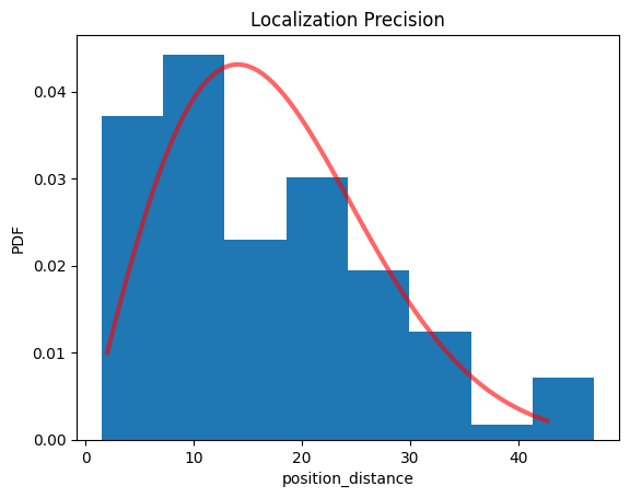
pipe.lp.results.head()

	position_delta_x	position_delta_y	position_distance	frame
0	-11.189941	4.859863	12.199716	24
1	32.580078	4.170410	32.845909	25
2	13.549805	-15.439941	20.542370	141
3	4.669922	3.010254	5.556060	142
4	20.469727	14.750000	25.230383	239

pipe.lp.hist();
print(pipe.lp.distribution_statistics.parameter_dict())

{'position_delta_x_loc': 0.6029139, 'position_delta_x_scale': 13.2682, 'position_delta_y_loc': -1.227687, 'position_delta_y_scale': 14.76087, 'position_distance_sigma': 14.067675781250028, 'position_distance_loc': 0, 'position_distance_scale': 1}

../../_images/c298ea8f2fff75a057c004029fb78db9cd090d26dad758b3eef9d4bd426ad1da.png

You can recover the computation procedure:

pipe.computation_as_string()

'def computation(self, locdata, n_localizations_min=4):\n    \n    # import required modules\n    from locan.analysis import LocalizationPrecision\n    \n    # prologue\n    self.file_indicator = locdata.meta.file.path\n    self.locdata = locdata\n    \n    # check requirements\n    if len(locdata)<=n_localizations_min:\n        return None\n    \n    # compute localization precision\n    self.lp = LocalizationPrecision().compute(self.locdata)\n    \n    return self\n'

or save it as text protocol:

The Pipeline object is pickleable and can thus be saved for revisits.

Apply the pipeline on multiple datasets - a batch process#

Let’s create multiple datasets:

path = lc.ROOT_DIR / 'tests/test_data/npc_gp210.asdf'
print(path, '\n')
dat = lc.load_locdata(path=path, file_type=lc.FileType.ASDF)

locdatas = [lc.select_by_condition(dat, f'{min}<index<{max}') for min, max in ((0,100), (101,202))]
locdatas

/home/docs/checkouts/readthedocs.org/user_builds/locan/envs/latest/lib/python3.11/site-packages/locan/tests/test_data/npc_gp210.asdf 

[<locan.data.locdata.LocData at 0x7f677aafa710>,
 <locan.data.locdata.LocData at 0x7f677a3209d0>]

Run the analysis pipeline as batch process

pipes = [lc.Pipeline(computation=computation, locdata=dat).compute() for dat in locdatas]

Processed frames::   0%|          | 0/6164 [00:00<?, ?it/s]

Processed frames::  18%|█▊        | 1113/6164 [00:00<00:00, 10409.72it/s]

Processed frames::  35%|███▍      | 2154/6164 [00:00<00:00, 8618.86it/s] 

Processed frames::  49%|████▉     | 3032/6164 [00:00<00:00, 8644.71it/s]

Processed frames::  63%|██████▎   | 3906/6164 [00:00<00:00, 8622.60it/s]

Processed frames::  77%|███████▋  | 4774/6164 [00:00<00:00, 7723.44it/s]

Processed frames:: 100%|██████████| 6164/6164 [00:00<00:00, 9060.59it/s]

Processed frames::   0%|          | 0/18639 [00:00<?, ?it/s]

Processed frames::   4%|▍         | 721/18639 [00:00<00:02, 6777.17it/s]

Processed frames::  11%|█         | 2005/18639 [00:00<00:01, 9743.37it/s]

Processed frames::  19%|█▉        | 3632/18639 [00:00<00:01, 12480.74it/s]

Processed frames::  32%|███▏      | 5936/18639 [00:00<00:00, 16008.57it/s]

Processed frames::  56%|█████▋    | 10512/18639 [00:00<00:00, 26183.89it/s]

Processed frames::  73%|███████▎  | 13645/18639 [00:00<00:00, 27881.09it/s]

Processed frames:: 100%|██████████| 18639/18639 [00:00<00:00, 33936.77it/s]

Processed frames:: 100%|██████████| 18639/18639 [00:00<00:00, 25282.72it/s]

As long as the batch procedure runs in a single computer process, the identifier increases with every instantiation.

[pipe.meta.identifier for pipe in pipes]

['2', '3']

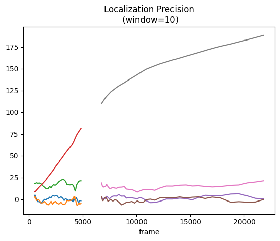
Visualize the combined results#

fig, ax = plt.subplots(nrows=1, ncols=1)
for pipe in pipes:
    pipe.lp.plot(ax=ax, window=10)
plt.show()

../../_images/d0559641e0f2805be4658c5b5558b67e9496c43cbd89ef60be9aae7c5f6460f5.png