Tutorial about computing hulls for localization data

For each set of localizations with 2D or 3D spatial coordinates various hull can be computed. A hull can be the minimal bounding box, the oriented minimal bounding box, the convex hull, or an alpha shape.

You can trigger computation of specific hull objects using a specific hull class or from the corresponding LocData attribute.

from pathlib import Path

%matplotlib inline

import numpy as np
import pandas as pd
import matplotlib.pyplot as plt

import locan as lc
from locan.data.hulls import BoundingBox, ConvexHull, OrientedBoundingBox

Jupyter environment detected. Enabling Open3D WebVisualizer.
[Open3D INFO] WebRTC GUI backend enabled.
[Open3D INFO] WebRTCWindowSystem: HTTP handshake server disabled.

lc.show_versions(system=False, dependencies=False, verbose=False)

Locan:
   version: 0.22.0.dev32+g4bfc3ab8b

Python:
   version: 3.11.14

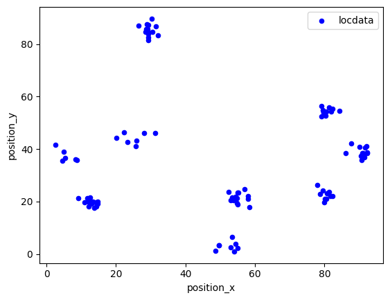
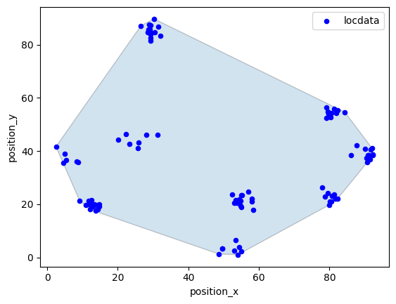
Synthetic data

rng = np.random.default_rng(seed=1)

locdata = lc.simulate_Thomas(parent_intensity=1e-3, region=((0, 100), (0, 100)), cluster_mu=10, cluster_std=2, seed=rng)

locdata.print_summary()

identifier: "1"
comment: ""
source: SIMULATION
state: RAW
element_count: 100
frame_count: 0
creation_time {
  2026-04-30T08:37:56.024288Z
}

fig, ax = plt.subplots(nrows=1, ncols=1)
locdata.data.plot.scatter(x='position_x', y='position_y', ax=ax, color='Blue', label='locdata')
plt.show()

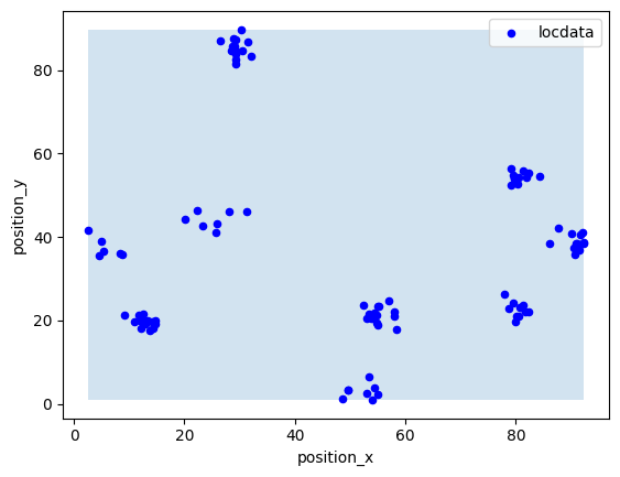
Minimal bounding box for spatial coordinates

# H = BoundingBox(locdata.coordinates)

H = locdata.bounding_box

print('dimension: ', H.dimension)
print('hull: ', H.hull)
print('width: ', H.width)
print('vertices: ', H.vertices)
print('region_measure: ', H.region_measure)
print('subregion_measure: ', H.subregion_measure)
print('region: ', H.region)

dimension:  2
hull:  [[ 2.490921    1.02997497]
 [92.36001123 89.71010693]]
width:  [89.86909023 88.68013196]
vertices:  [[ 2.490921   92.36001123]
 [ 1.02997497 89.71010693]]
region_measure:  7969.602780428899
subregion_measure:  357.0984443733635
region:  AxisOrientedRectangle((2.490921001041831, 1.0299749716244107), 89.86909022532446, 88.6801319613573)

fig, ax = plt.subplots(nrows=1, ncols=1)
ax.add_patch(locdata.bounding_box.region.as_artist(alpha=0.2))
locdata.data.plot.scatter(x='position_x', y='position_y', ax=ax, color='Blue', label='locdata')
plt.show()

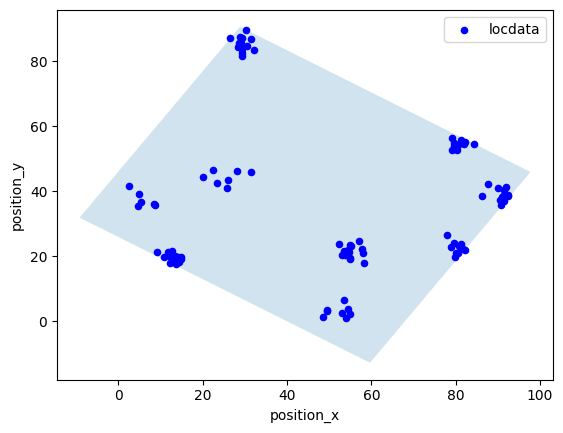
Oriented minimal bounding box for spatial coordinates

# H = OrientedBoundingBox(locdata.coordinates)

H = locdata.oriented_bounding_box

print('dimension: ', H.dimension)
print('hull: ', H.hull)
print('vertices: ', H.vertices)
print('width: ', H.width)
print('region_measure: ', H.region_measure)
print('subregion_measure: ', H.subregion_measure)
print('region: ', H.region)

dimension:  2
hull:  POLYGON ((-9.220392369565374 31.865082145844063, 28.845458559801138 90.5971273151963, 97.75586149761332 45.9344032750304, 59.69001056824682 -12.797641894321849, -9.220392369565374 31.865082145844063))
vertices:  [[ -9.22039237  31.86508215]
 [ 28.84545856  90.59712732]
 [ 97.7558615   45.93440328]
 [ 59.69001057 -12.79764189]
 [ -9.22039237  31.86508215]]
width:  [82.11822302 69.9890144 ]
region_measure:  5747.37349339424
subregion_measure:  304.2144748382608
region:  Rectangle((-9.220392369565374, 31.865082145844063), 82.11822301864336, 69.98901440048706, -32.9483801916185)

fig, ax = plt.subplots(nrows=1, ncols=1)
ax.add_patch(locdata.oriented_bounding_box.region.as_artist(alpha=0.2))
locdata.data.plot.scatter(x='position_x', y='position_y', ax=ax, color='Blue', label='locdata')
plt.show()

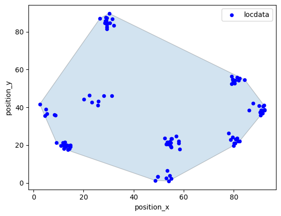
Convex hull

Convex hull for spatial coordinates (scipy)

# H = ConvexHull(locdata.coordinates, method='scipy')

H = locdata.convex_hull

print('dimension: ', H.dimension)
print('hull: ', H.hull)
# print('vertex_indices: ', H.vertex_indices)
# print('vertices: ', H.vertices)
print('region_measure: ', H.region_measure)
print('subregion_measure: ', H.subregion_measure)
print('points on boundary: ', H.points_on_boundary)
print('points on boundary relative to all points: ', H.points_on_boundary_rel)
print('region: ', H.region)

dimension:  2
hull:  <scipy.spatial._qhull.ConvexHull object at 0x72bbc84b3950>
region_measure:  4908.170783871255
subregion_measure:  264.4870519254037
points on boundary:  13
points on boundary relative to all points:  0.13
region:  Polygon(<self.vertices>, <self.holes>)

fig, ax = plt.subplots(nrows=1, ncols=1)
ax.add_patch(locdata.convex_hull.region.as_artist(alpha=0.2))
locdata.data.plot.scatter(x='position_x', y='position_y', ax=ax, color='Blue', label='locdata')
plt.show()

Convex hull for spatial coordinates (shapely)

Some hulls can be computed from different algorithms. If implemented, use the methods parameter to specify the algorithm.

H = ConvexHull(locdata.coordinates, method='shapely')

print('dimension: ', H.dimension)
print('hull: ', H.hull)
# print('vertices: ', H.vertices)
print('region_measure: ', H.region_measure)
print('subregion_measure: ', H.subregion_measure)
print('points on boundary: ', H.points_on_boundary)
print('points on boundary relative to all points: ', H.points_on_boundary_rel)
print('region: ', H.region)

dimension:  2
hull:  POLYGON ((54.029321929694525 1.0299749716244107, 48.634206414428576 1.294631346507537, 12.175420163612081 17.997868633149913, 9.18991822286495 21.36788078938049, 2.490921001041831 41.64287079543503, 26.54041545299338 87.040661544405, 30.214047987922243 89.71010693298172, 84.34954910628653 54.62340239857981, 91.9734281153137 41.17838012011845, 92.33940616216016 38.808549274650204, 92.36001122636628 38.48950874170735, 82.28290378326082 22.061077730066597, 79.83990217703906 19.69136737327613, 54.029321929694525 1.0299749716244107))
region_measure:  4908.170783871255
subregion_measure:  264.4870519254038
points on boundary:  13
points on boundary relative to all points:  0.13
region:  Polygon(<self.vertices>, <self.holes>)

fig, ax = plt.subplots(nrows=1, ncols=1)
ax.add_patch(H.region.as_artist(alpha=0.2))
locdata.data.plot.scatter(x='position_x', y='position_y', ax=ax, color='Blue', label='locdata')
plt.show()

Alpha shape for spatial coordinates

The alpha shape depends on a single parameter alpha (not to confuse with the alpha to specify opacity in figures). The alpha complex is an alpha-independent representation of all alpha shapes.

You can get all apha values for which the corresponding alpha shape changes.

lc.AlphaComplex(locdata.coordinates).alphas()

array([4.79010715e-02, 6.26886019e-02, 9.00848038e-02, 1.26327560e-01,
       1.27719280e-01, 1.35082505e-01, 1.48065929e-01, 1.59852612e-01,
       1.80345970e-01, 2.29967352e-01, 2.38528055e-01, 2.40927392e-01,
       2.41691338e-01, 2.66695006e-01, 2.77822554e-01, 2.94376165e-01,
       3.06743479e-01, 3.25282310e-01, 3.38425410e-01, 3.43041012e-01,
       3.43184730e-01, 3.52204265e-01, 3.57124009e-01, 3.58975685e-01,
       3.62059409e-01, 3.74195019e-01, 3.78291044e-01, 3.97084183e-01,
       4.00186670e-01, 4.02716245e-01, 4.02815627e-01, 4.03838992e-01,
       4.09114331e-01, 4.18957692e-01, 4.19626534e-01, 4.33534796e-01,
       4.47358936e-01, 4.47427686e-01, 4.50668384e-01, 4.56413180e-01,
       4.67180830e-01, 4.71727787e-01, 4.75216918e-01, 4.81997429e-01,
       4.82164830e-01, 4.83113289e-01, 4.97024836e-01, 4.99990289e-01,
       5.06241764e-01, 5.08056086e-01, 5.13965130e-01, 5.25320369e-01,
       5.31023418e-01, 5.34700206e-01, 5.39200680e-01, 5.49324870e-01,
       5.53496939e-01, 5.58987615e-01, 5.59448067e-01, 5.59889793e-01,
       5.61663190e-01, 5.67027377e-01, 5.67749948e-01, 5.71279300e-01,
       5.79365256e-01, 5.81283629e-01, 5.92103004e-01, 5.97516286e-01,
       6.00674458e-01, 6.01810488e-01, 6.03537738e-01, 6.06574504e-01,
       6.06739584e-01, 6.09413711e-01, 6.10475779e-01, 6.12372458e-01,
       6.18571992e-01, 6.19901061e-01, 6.20713067e-01, 6.24413788e-01,
       6.40082879e-01, 6.43856168e-01, 6.51568398e-01, 6.62544191e-01,
       6.64871359e-01, 6.82998920e-01, 6.89013581e-01, 6.89804375e-01,
       6.95662528e-01, 6.96671784e-01, 6.97171260e-01, 7.00419524e-01,
       7.00672239e-01, 7.09863544e-01, 7.11029883e-01, 7.12728093e-01,
       7.15296258e-01, 7.18750000e-01, 7.21811422e-01, 7.28198767e-01,
       7.34206960e-01, 7.37019513e-01, 7.38740770e-01, 7.39835123e-01,
       7.40429317e-01, 7.41294381e-01, 7.46229214e-01, 7.49077113e-01,
       7.50780227e-01, 7.51443768e-01, 7.58053002e-01, 7.59059846e-01,
       7.60024130e-01, 7.61763351e-01, 7.62189329e-01, 7.63885515e-01,
       7.68648386e-01, 7.69917786e-01, 7.72450447e-01, 7.73355937e-01,
       7.84442099e-01, 7.89951563e-01, 7.91274054e-01, 7.93343902e-01,
       7.94881105e-01, 7.99868788e-01, 8.03569058e-01, 8.11065191e-01,
       8.22856563e-01, 8.25319529e-01, 8.26052181e-01, 8.33933862e-01,
       8.39957725e-01, 8.44739640e-01, 8.45339954e-01, 8.46103046e-01,
       8.49229872e-01, 8.50666106e-01, 8.51344679e-01, 8.52808232e-01,
       8.53924453e-01, 8.56196465e-01, 8.62069666e-01, 8.69376152e-01,
       8.70348990e-01, 8.79922419e-01, 8.83510627e-01, 8.88291895e-01,
       8.89253318e-01, 8.90296830e-01, 9.03293099e-01, 9.03545920e-01,
       9.05171752e-01, 9.14296150e-01, 9.15013552e-01, 9.19769930e-01,
       9.21676338e-01, 9.25606663e-01, 9.42225183e-01, 9.53726892e-01,
       9.60651636e-01, 9.66079966e-01, 9.79994236e-01, 9.82761562e-01,
       9.85767096e-01, 9.88304664e-01, 9.93925311e-01, 9.98617093e-01,
       1.01493196e+00, 1.01742625e+00, 1.01790607e+00, 1.02895805e+00,
       1.02982855e+00, 1.03053951e+00, 1.03230173e+00, 1.03420508e+00,
       1.03951764e+00, 1.04708194e+00, 1.04779857e+00, 1.05280507e+00,
       1.06181049e+00, 1.06634542e+00, 1.06639910e+00, 1.08017528e+00,
       1.08501873e+00, 1.09518923e+00, 1.09869778e+00, 1.10539327e+00,
       1.11120765e+00, 1.11301014e+00, 1.11431563e+00, 1.11952155e+00,
       1.13356306e+00, 1.13472354e+00, 1.13733855e+00, 1.15128479e+00,
       1.15750823e+00, 1.16736695e+00, 1.16926401e+00, 1.17387209e+00,
       1.18544233e+00, 1.18551348e+00, 1.19242406e+00, 1.19896186e+00,
       1.20048927e+00, 1.20720985e+00, 1.23595162e+00, 1.23873969e+00,
       1.25545681e+00, 1.25617021e+00, 1.26070725e+00, 1.26166427e+00,
       1.26240010e+00, 1.26532192e+00, 1.27488250e+00, 1.27724424e+00,
       1.28234004e+00, 1.28505528e+00, 1.29847419e+00, 1.30029954e+00,
       1.31068196e+00, 1.31351678e+00, 1.31691837e+00, 1.31732738e+00,
       1.33458446e+00, 1.33516061e+00, 1.34370910e+00, 1.34592843e+00,
       1.34663685e+00, 1.34918952e+00, 1.36000347e+00, 1.36376810e+00,
       1.36698663e+00, 1.36752224e+00, 1.41311264e+00, 1.42226765e+00,
       1.42590427e+00, 1.43529046e+00, 1.43628331e+00, 1.45069543e+00,
       1.46575487e+00, 1.48152517e+00, 1.48366972e+00, 1.48798907e+00,
       1.49018192e+00, 1.52334060e+00, 1.52581942e+00, 1.52870001e+00,
       1.53542071e+00, 1.53856671e+00, 1.54411054e+00, 1.54584873e+00,
       1.55976987e+00, 1.57562096e+00, 1.58411018e+00, 1.61295349e+00,
       1.61741832e+00, 1.62776308e+00, 1.63309288e+00, 1.63940332e+00,
       1.64733370e+00, 1.65626521e+00, 1.65801787e+00, 1.66668296e+00,
       1.69711226e+00, 1.70174793e+00, 1.71063423e+00, 1.71714404e+00,
       1.72508327e+00, 1.73141334e+00, 1.73767984e+00, 1.74668941e+00,
       1.74748707e+00, 1.75132489e+00, 1.75463569e+00, 1.77157747e+00,
       1.77362769e+00, 1.77744793e+00, 1.78223117e+00, 1.78501180e+00,
       1.79207963e+00, 1.79918946e+00, 1.80006516e+00, 1.82414077e+00,
       1.82525146e+00, 1.87382782e+00, 1.89365721e+00, 1.91381607e+00,
       1.92656279e+00, 1.94884908e+00, 2.00579000e+00, 2.01728998e+00,
       2.03034431e+00, 2.04412985e+00, 2.05045009e+00, 2.05349095e+00,
       2.07286096e+00, 2.16816869e+00, 2.20910083e+00, 2.22506809e+00,
       2.24795084e+00, 2.25112215e+00, 2.27054590e+00, 2.27811322e+00,
       2.27983143e+00, 2.31343855e+00, 2.32264410e+00, 2.32880977e+00,
       2.34437490e+00, 2.37715769e+00, 2.37718224e+00, 2.38285089e+00,
       2.39569231e+00, 2.41101384e+00, 2.43547082e+00, 2.45665550e+00,
       2.45903945e+00, 2.52246605e+00, 2.54217362e+00, 2.62136822e+00,
       2.65109801e+00, 2.65969443e+00, 2.70080147e+00, 2.79517221e+00,
       2.84755996e+00, 2.85698318e+00, 2.90440130e+00, 3.01656649e+00,
       3.07917748e+00, 3.13521767e+00, 3.17768097e+00, 3.26467278e+00,
       3.38251472e+00, 3.56989360e+00, 3.57573605e+00, 3.59266281e+00,
       3.60196066e+00, 3.63035035e+00, 3.69906825e+00, 3.95778513e+00,
       4.26390743e+00, 4.29838037e+00, 4.90186930e+00, 4.97166061e+00,
       6.07922626e+00, 6.24118004e+00, 6.24886703e+00, 6.35586273e+00,
       6.39866293e+00, 6.48269939e+00, 6.65001925e+00, 6.94378885e+00,
       7.14344811e+00, 7.21201452e+00, 7.24911348e+00, 7.26452608e+00,
       7.32337306e+00, 7.41191471e+00, 7.42595673e+00, 7.43392888e+00,
       7.43433571e+00, 7.72806825e+00, 7.74336647e+00, 7.76088428e+00,
       7.78952885e+00, 7.80165047e+00, 7.82651854e+00, 7.85021562e+00,
       7.87716234e+00, 7.88720512e+00, 7.96645164e+00, 8.04566727e+00,
       8.08224562e+00, 8.09483397e+00, 8.26561737e+00, 8.31590652e+00,
       8.51343155e+00, 8.71703225e+00, 8.74628027e+00, 8.79369640e+00,
       8.94187403e+00, 8.95071004e+00, 9.00003433e+00, 9.01593685e+00,
       9.63640804e+00, 9.86225891e+00, 1.01897890e+01, 1.02221135e+01,
       1.02751450e+01, 1.03599520e+01, 1.03913298e+01, 1.04465878e+01,
       1.04471321e+01, 1.04597259e+01, 1.05636147e+01, 1.05639095e+01,
       1.05738659e+01, 1.06432228e+01, 1.06765138e+01, 1.08061930e+01,
       1.08267384e+01, 1.10126219e+01, 1.11019335e+01, 1.17944937e+01,
       1.17991457e+01, 1.19695055e+01, 1.20037985e+01, 1.21184540e+01,
       1.22847881e+01, 1.30919383e+01, 1.50017576e+01, 1.51307502e+01,
       1.53817915e+01, 1.58322811e+01, 1.59250873e+01, 1.59542235e+01,
       1.59653788e+01, 1.66977766e+01, 1.75114155e+01, 1.76752204e+01,
       1.77796252e+01, 1.77821693e+01, 1.78396689e+01, 1.78495038e+01,
       1.78527508e+01, 1.80088272e+01, 1.87142131e+01, 1.89454045e+01,
       1.89693286e+01, 1.89963303e+01, 1.90443249e+01, 1.91047288e+01,
       1.91360626e+01, 1.91361599e+01, 1.91392739e+01, 1.91597195e+01,
       1.91653271e+01, 1.91703625e+01, 1.91811028e+01, 1.92761620e+01,
       1.94601021e+01, 1.96390972e+01, 2.00514415e+01, 2.02227230e+01,
       2.15705147e+01, 2.39869621e+01, 2.41473984e+01, 2.41540470e+01,
       2.44485075e+01, 2.46186829e+01, 2.56872419e+01, 2.63949127e+01,
       2.70955193e+01, 2.78667049e+01, 2.82256845e+01, 2.95858969e+01,
       2.98130741e+01, 3.06827051e+01, 3.22557333e+01, 3.70800591e+01,
       5.09825249e+01, 5.34146233e+01, 7.99051743e+01, 9.91221237e+01,
       1.42276382e+02, 4.34636383e+02, 4.71113129e+02, 1.32363586e+03,
                  inf])

You can determine an optimal alpha, i.e. the smallest alpha for which all points are still part of the alpha shape.

opt_alpha = lc.AlphaComplex(locdata.coordinates).optimal_alpha()
opt_alpha

np.float64(32.25573327495765)

# H = lc.AlphaShape(opt_alpha, locdata.coordinates)

locdata.update_alpha_shape(alpha=opt_alpha)
H = locdata.alpha_shape

print('dimension: ', H.dimension)
# print('vertex_indices: ', H.vertex_indices)
# print('vertices: ', H.vertices)
print('region_measure: ', H.region_measure)
print('subregion_measure: ', H.subregion_measure)
print('points in alpha shape: ', H.n_points_alpha_shape)
print('points in alpha shape relative to all points: ', H.n_points_alpha_shape_rel)
print('points on boundary: ', H.n_points_on_boundary)
print('points on boundary relative to all points: ', H.n_points_on_boundary_rel)
print('region: ', H.region)

dimension:  2
region_measure:  4908.1707838712555
subregion_measure:  264.4870519254038
points in alpha shape:  100
points in alpha shape relative to all points:  1.0
points on boundary:  22
points on boundary relative to all points:  0.22
region:  Polygon(<self.vertices>, <self.holes>)

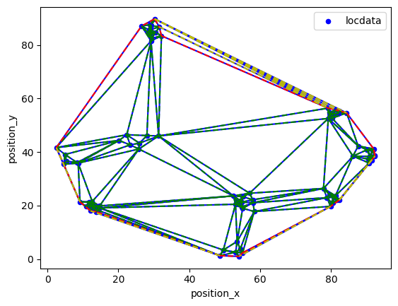
The alpha shape is made of different vertex types that can be differentiated as exterior, interior, regular or singular.

ac_simplices_all = H.alpha_complex.get_alpha_complex_lines(H.alpha, type='all')
ac_simplices_exterior = H.alpha_complex.get_alpha_complex_lines(H.alpha, type='exterior')
ac_simplices_interior = H.alpha_complex.get_alpha_complex_lines(H.alpha, type='interior')
ac_simplices_regular = H.alpha_complex.get_alpha_complex_lines(H.alpha, type='regular')
ac_simplices_singular = H.alpha_complex.get_alpha_complex_lines(H.alpha, type='singular')

fig, ax = plt.subplots(nrows=1, ncols=1)

for simp in ac_simplices_all:
    ax.plot(locdata.coordinates[simp, 0], locdata.coordinates[simp, 1], '-b')
for simp in ac_simplices_interior:
    ax.plot(locdata.coordinates[simp, 0], locdata.coordinates[simp, 1], '--g')
for simp in ac_simplices_regular:
    ax.plot(locdata.coordinates[simp, 0], locdata.coordinates[simp, 1], '--r')
for simp in ac_simplices_singular:
    ax.plot(locdata.coordinates[simp, 0], locdata.coordinates[simp, 1], '--y')

locdata.data.plot.scatter(x='position_x', y='position_y', ax=ax, color='Blue', label='locdata')
plt.show()

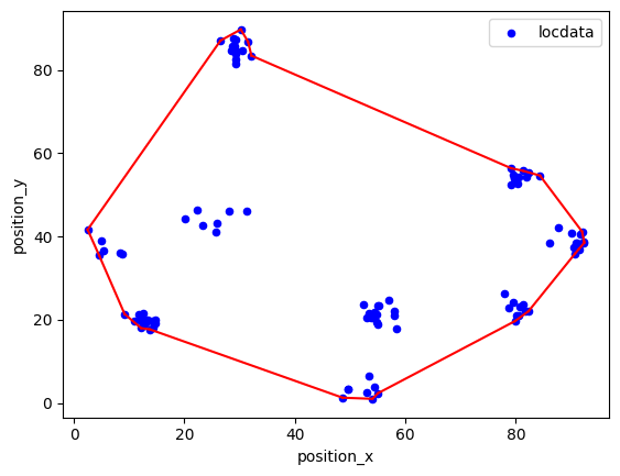
Often the regular representation is good enough.

fig, ax = plt.subplots(nrows=1, ncols=1)
for simp in ac_simplices_regular:
    ax.plot(locdata.coordinates[simp, 0], locdata.coordinates[simp, 1], '-r')
locdata.data.plot.scatter(x='position_x', y='position_y', ax=ax, color='Blue', label='locdata')
plt.show()

You can get the connected components as list of Region.

H.connected_components

[Polygon([[26.54041545299338, 87.040661544405], [30.214047987922243, 89.71010693298172], [84.34954910628653, 54.62340239857981], [91.9734281153137, 41.17838012011845], [92.33940616216016, 38.808549274650204], [92.36001122636628, 38.48950874170735], [82.28290378326082, 22.061077730066597], [79.83990217703906, 19.69136737327613], [54.029321929694525, 1.0299749716244107], [48.634206414428576, 1.294631346507537], [12.175420163612081, 17.997868633149913], [9.18991822286495, 21.36788078938049], [2.490921001041831, 41.64287079543503]], [])]

connected_component_0 = H.connected_components[0]

print('dimension: ', connected_component_0.dimension)
print('region_measure: ', connected_component_0.region_measure)
print('subregion_measure: ', connected_component_0.subregion_measure)

dimension:  2
region_measure:  4908.1707838712555
subregion_measure:  264.4870519254038

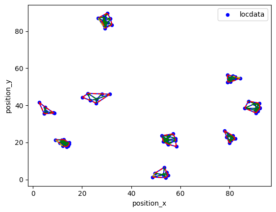
The alpha shape for a smaller alpha can have multiple connected components.

H = lc.AlphaShape(5, locdata.coordinates)

print('dimension: ', H.dimension)
# print('vertex_indices: ', H.vertex_indices)
# print('vertices: ', H.vertices)
print('region_measure: ', H.region_measure)
print('subregion_measure: ', H.subregion_measure)
print('points in alpha shape: ', H.n_points_alpha_shape)
print('points in alpha shape relative to all points: ', H.n_points_alpha_shape_rel)
print('points on boundary: ', H.n_points_on_boundary)
print('points on boundary relative to all points: ', H.n_points_on_boundary_rel)

dimension:  2
region_measure:  178.41254317639843
subregion_measure:  171.67742405936463
points in alpha shape:  100
points in alpha shape relative to all points:  1.0
points on boundary:  57
points on boundary relative to all points:  0.57

ac_simplices_all = H.alpha_complex.get_alpha_complex_lines(H.alpha, type='all')
ac_simplices_exterior = H.alpha_complex.get_alpha_complex_lines(H.alpha, type='exterior')
ac_simplices_interior = H.alpha_complex.get_alpha_complex_lines(H.alpha, type='interior')
ac_simplices_regular = H.alpha_complex.get_alpha_complex_lines(H.alpha, type='regular')
ac_simplices_singular = H.alpha_complex.get_alpha_complex_lines(H.alpha, type='singular')

fig, ax = plt.subplots(nrows=1, ncols=1)

for simp in ac_simplices_all:
    ax.plot(locdata.coordinates[simp, 0], locdata.coordinates[simp, 1], '-b')
for simp in ac_simplices_interior:
    ax.plot(locdata.coordinates[simp, 0], locdata.coordinates[simp, 1], '--g')
for simp in ac_simplices_regular:
    ax.plot(locdata.coordinates[simp, 0], locdata.coordinates[simp, 1], '--r')
for simp in ac_simplices_singular:
    ax.plot(locdata.coordinates[simp, 0], locdata.coordinates[simp, 1], '--y')

locdata.data.plot.scatter(x='position_x', y='position_y', ax=ax, color='Blue', label='locdata')
plt.show()

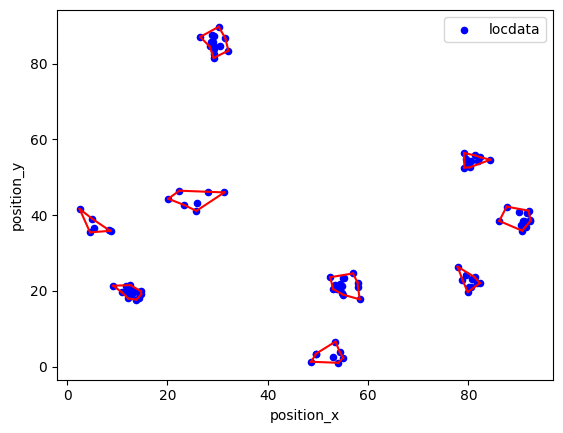
The regular representation:

fig, ax = plt.subplots(nrows=1, ncols=1)
for simp in ac_simplices_regular:
    ax.plot(locdata.coordinates[simp, 0], locdata.coordinates[simp, 1], '-r')
locdata.data.plot.scatter(x='position_x', y='position_y', ax=ax, color='Blue', label='locdata')
plt.show()

The connected components:

H.connected_components

[Polygon([[4.574030584926964, 35.4547363609949], [2.490921001041831, 41.64287079543503], [4.957382196904078, 39.08282122381802], [8.355461487809666, 36.04765129727869], [8.66131719294932, 35.8564682341916]], []),
 Polygon([[25.770117329307787, 41.124276031608815], [23.31756949147803, 42.6744624631213], [20.173587957294433, 44.31714346765541], [22.361223833116604, 46.453014294097834], [28.048700032796415, 46.15804762285728], [31.339293507790977, 45.9942555369238]], []),
 Polygon([[9.18991822286495, 21.36788078938049], [12.636282213847565, 21.529820077010385], [14.734872660721315, 19.880462363217678], [14.769094009431546, 19.124654613922488], [14.266019685598483, 18.241818179484355], [13.747576761626673, 17.702091783845788], [12.175420163612081, 17.997868633149913]], []),
 Polygon([[26.54041545299338, 87.040661544405], [30.214047987922243, 89.71010693298172], [31.521384860659595, 86.75121552412102], [32.14133335513356, 83.41408741528058], [29.20688463095611, 81.48951050894098]], []),
 Polygon([[79.18789302054475, 52.543982100600005], [79.11703202181116, 56.39645603252982], [81.32782142473194, 55.75284367902573], [84.34954910628653, 54.62340239857981], [80.25475558909794, 52.61761293856212]], []),
 Polygon([[87.6064843703255, 42.247461144808746], [91.9734281153137, 41.17838012011845], [92.33940616216016, 38.808549274650204], [92.36001122636628, 38.48950874170735], [91.40098079916173, 36.989250622930314], [90.7011218417029, 35.889994988035625], [86.13341308357771, 38.463382259593324]], []),
 Polygon([[54.029321929694525, 1.0299749716244107], [48.634206414428576, 1.294631346507537], [49.59358344008751, 3.4015003371361145], [53.482683026695234, 6.614947738231005], [54.37183424361821, 3.788452129115082], [55.03000267597442, 2.3642990669580453]], []),
 Polygon([[53.02310815665912, 20.494919113980316], [52.4417533406316, 23.609344720491215], [56.99055629523848, 24.610250050117035], [57.896406888972834, 22.172515398810596], [57.98560316805971, 21.06912087658576], [58.31284235106916, 17.772793788937257], [55.04194051962414, 18.999536120747145]], []),
 Polygon([[78.79284317381992, 22.962147412197464], [77.83372328947765, 26.395146222813697], [81.19928424977152, 23.660768547251035], [82.28290378326082, 22.061077730066597], [79.83990217703906, 19.69136737327613]], [])]

connected_component_0 = H.connected_components[0]

print('dimension: ', connected_component_0.dimension)
print('region_measure: ', connected_component_0.region_measure)
print('subregion_measure: ', connected_component_0.subregion_measure)

dimension:  2
region_measure:  12.16313947011497
subregion_measure:  19.10814169604162