Tutorial about analyzing grouped cluster properties
Localization properties vary within clusters. Analyzing such variations can help to characterize cluster populations. Here, we show examples for variations in convex hull properties or coordinate variances.
from pathlib import Path

%matplotlib inline

import numpy as np
import pandas as pd
import matplotlib.pyplot as plt
from colorcet import m_fire, m_gray, m_dimgray

import locan as lc
lc.show_versions(system=False, dependencies=False, verbose=False)
Locan:
   version: 0.22.0.dev32+g4bfc3ab8b

Python:
   version: 3.11.14
Synthetic data
We simulate localization data that follows a Neyman-Scott distribution in 2D:
rng = np.random.default_rng(seed=1)
locdata = lc.simulate_dstorm(parent_intensity=1e-5, region=((0, 10_000), (0, 10_000)), cluster_mu=10, cluster_std=10, seed=rng)

locdata.print_summary()
Jupyter environment detected. Enabling Open3D WebVisualizer.
[Open3D INFO] WebRTC GUI backend enabled.
[Open3D INFO] WebRTCWindowSystem: HTTP handshake server disabled.
identifier: "1"
comment: ""
source: SIMULATION
state: RAW
element_count: 10380
frame_count: 0
creation_time {
  2026-04-30T08:34:04.857006Z
}
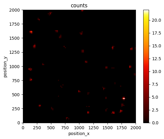
bin_range=((0, 2_000), (0, 2_000))
lc.render_2d_mpl(locdata, bin_size=20, bin_range=bin_range)
<Axes: title={'center': 'counts'}, xlabel='position_x', ylabel='position_y'>
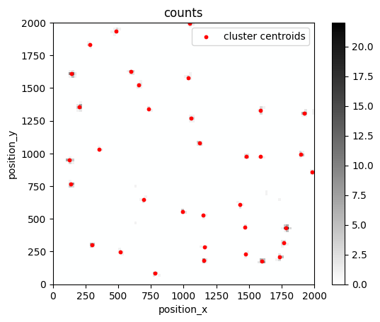
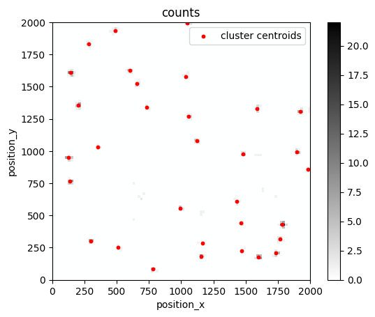
True clusters
First we look at ground truth clusters.
grouped = locdata.data.groupby("cluster_label")
clust = lc.LocData.from_collection([lc.LocData.from_selection(locdata, indices=group.index) for name, group in grouped])
Filter out clusters with less than 3 localizations since on convex hull can be computed for such clusters.
clust_selection = lc.select_by_condition(clust, condition="2 < localization_count")
references_ = [clust.references[i] for i in clust_selection.indices]
clust_selection.reduce()
clust_selection.references = references_
clust = clust_selection
Show code cell source
n_clustered_loc = np.sum([ref.properties['localization_count'] for ref in clust.references])
print(f"Number of clusters: {clust.properties['localization_count']}")
print(f"Number of clustered localizations: {n_clustered_loc}")
print(f"Ratio cluster to noise localizations: {n_clustered_loc / len(locdata):.3}")
Number of clusters: 771
Number of clustered localizations: 10172
Ratio cluster to noise localizations: 0.98
fig, ax = plt.subplots(nrows=1, ncols=1)
lc.render_2d_mpl(locdata, bin_size=20, bin_range=bin_range, cmap=m_gray.reversed())
clust.data.plot.scatter(x='position_x', y='position_y', ax=ax, color='Red', s=10, label='cluster centroids', xlim=bin_range[0], ylim=bin_range[1])
plt.show()
clust.data.head()
| localization_count | position_x | uncertainty_x | position_y | uncertainty_y | region_measure_bb | localization_density_bb | subregion_measure_bb | region_measure | localization_density | subregion_measure | |
|---|---|---|---|---|---|---|---|---|---|---|---|
| 0 | 24 | 1399.549521 | 1.877356 | 9539.052779 | 1.853978 | 1025.930045 | 0.023393 | 128.121678 | 100000000 | 2.400000e-07 | 40000 |
| 2 | 3 | 8303.079096 | 10.889812 | 4081.419445 | 3.852366 | 456.241155 | 0.006575 | 96.259339 | 100000000 | 3.000000e-08 | 40000 |
| 3 | 7 | 5507.141828 | 2.444467 | 224.387484 | 2.132102 | 336.278485 | 0.020816 | 73.989892 | 100000000 | 7.000000e-08 | 40000 |
| 4 | 4 | 7561.723474 | 3.515554 | 5385.880528 | 5.842642 | 443.103490 | 0.009027 | 87.512555 | 100000000 | 4.000000e-08 | 40000 |
| 5 | 7 | 3279.865197 | 5.284643 | 7918.206789 | 2.848332 | 774.964110 | 0.009033 | 117.649012 | 100000000 | 7.000000e-08 | 40000 |
clust.properties
{'localization_count': 771,
 'position_x': np.float64(5078.461816893804),
 'uncertainty_x': np.float64(138.598117645907),
 'position_y': np.float64(5571.31780554545),
 'uncertainty_y': np.float64(421.90449657593706),
 'region_measure_bb': np.float64(99518129.6386362),
 'localization_density_bb': np.float64(7.7473320971727e-06),
 'subregion_measure_bb': np.float64(39903.55763820844)}
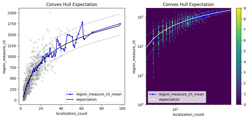
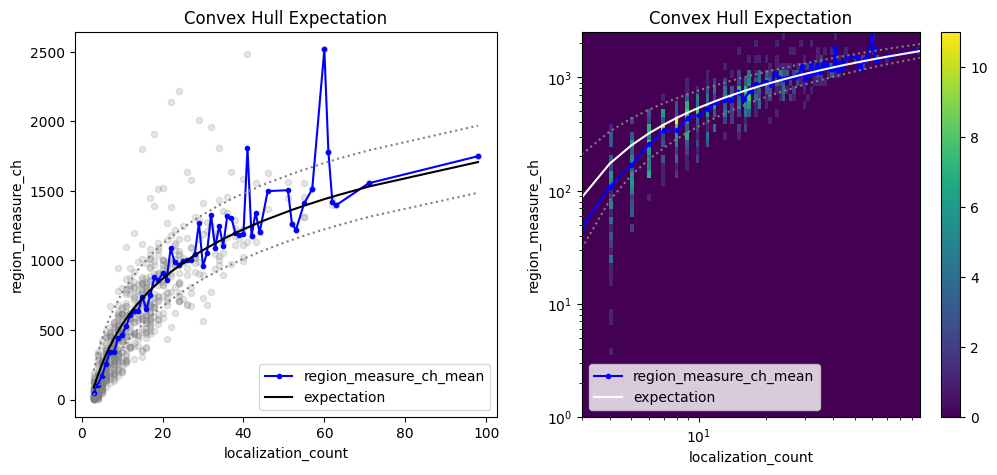
Investigate the convex hull areas
Localization clusters can be analyzed with respect to their convex hull region properties as function of localization_count as outlined in Ebert et al. (https://doi:10.1093/bioinformatics/btac700).
che = lc.ConvexHullExpectation(convex_hull_property='region_measure_ch', expected_variance=10**2).compute(locdata=clust)
che.results
<locan.analysis.convex_hull_expectation.ConvexHullExpectationResults at 0x7d27e9d48810>
fig, axes = plt.subplots(nrows=1, ncols=2, figsize=(12, 5))
che.plot(ax=axes[0])
che.hist(ax=axes[1]);
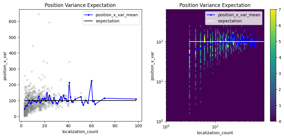
Investigate the position variances
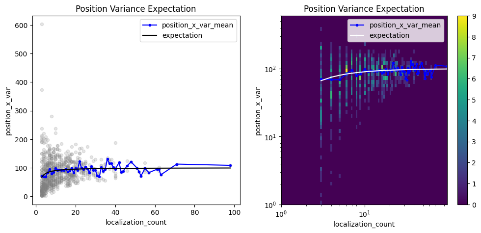
Localization coordinates in localization clusters come with a certain variance. The variance is related to the localization precision or other localization properties but also varies with localization_count if determined as biased sample variance (i.e. without Bessel’s correction).
pve_biased = lc.PositionVarianceExpectation(loc_property="position_x", expectation=10**2, biased=True).compute(locdata=clust)
pve_biased.results
<locan.analysis.position_variance_expectation.PositionVarianceExpectationResults at 0x7d27ea39a0d0>
fig, axes = plt.subplots(nrows=1, ncols=2, figsize=(12, 5))
pve_biased.plot(ax=axes[0])
pve_biased.hist(ax=axes[1]);
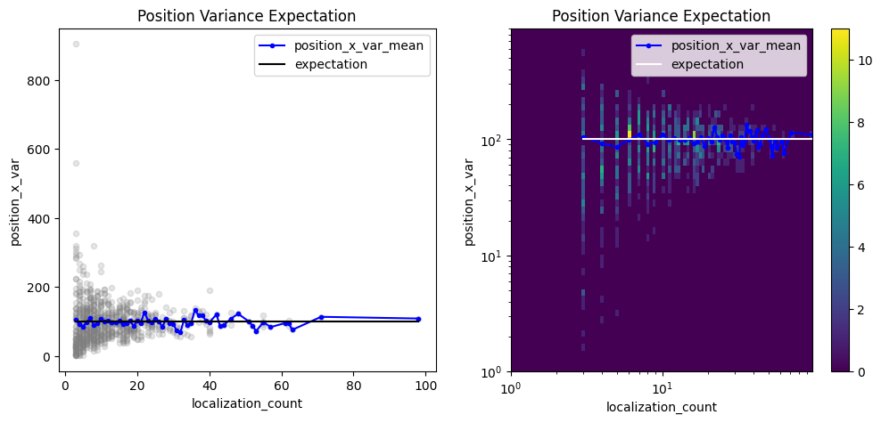
A similar analysis can be performed with unbiased variances in which Bessel’s correction is applied.
pve = lc.PositionVarianceExpectation(loc_property="position_x", expectation=10**2, biased=False).compute(locdata=clust)
pve.results
<locan.analysis.position_variance_expectation.PositionVarianceExpectationResults at 0x7d27e340b810>
fig, axes = plt.subplots(nrows=1, ncols=2, figsize=(12, 5))
pve.plot(ax=axes[0])
pve.hist(ax=axes[1], log=True);
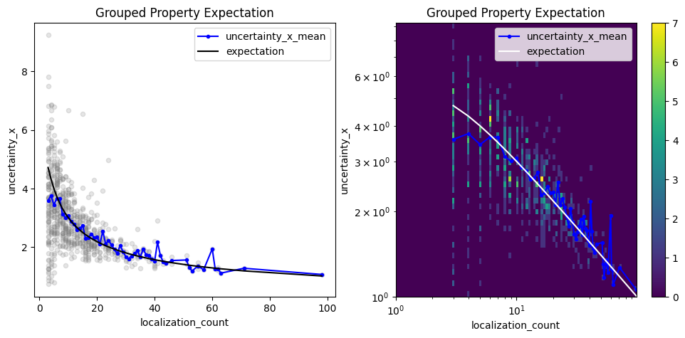
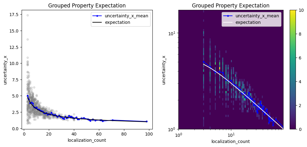
Investigate any grouped property
A similar analysis can be carried out with any LocData property. For instance, let’s check the coordinate uncertainties of cluster centroids. The uncertainty in one dimension should follow the square root of the biased position variance for clusters with variable number of localizations.
It is important to consider the differences between variance and standard deviation. Position uncertainties are usually given as standard deviation with units equal to position units. Converting the ground truth for the coordinate standard deviation in each cluster (std as used in the simulations above) requires a Bessel correction on the squared std being the variance). In addition the coordinate uncertainties of cluster centroids should scale with the inverse square root of the number of localizations per cluster.
n_locs = np.arange(1, 1000)
ground_truth_std = 10
ground_truth_variance = ground_truth_std**2
biased_variance = ground_truth_variance * (1 - 1 / n_locs)
biased_uncertainty = np.sqrt(biased_variance)
expected_uncertainty = biased_uncertainty / np.sqrt(n_locs)
expectation = pd.Series(data=expected_uncertainty, index=n_locs)
expectation;
loc_property = "uncertainty_x"
other_loc_property = "localization_count"
gpe = lc.GroupedPropertyExpectation(loc_property=loc_property, other_loc_property=other_loc_property, expectation=expectation).compute(locdata=clust)
gpe.results
<locan.analysis.grouped_property_expectation.GroupedPropertyExpectationResults at 0x7d27e99ee190>
fig, axes = plt.subplots(nrows=1, ncols=2, figsize=(12, 5))
gpe.plot(ax=axes[0])
gpe.hist(ax=axes[1]);
Cluster localizations by dbscan
When clustering data by dbscan slight deviations appear between expectation and computed properties.
noise, clust = lc.cluster_dbscan(locdata, eps=20, min_samples=3)
Show code cell source
n_clustered_loc = np.sum([ref.properties['localization_count'] for ref in clust.references])
print(f"Number of clusters: {clust.properties['localization_count']}")
print(f"Number of noise localizations: {noise.properties['localization_count']}")
print(f"Number of clustered localizations: {n_clustered_loc}")
print(f"Ratio cluster to noise localizations: {n_clustered_loc / (n_clustered_loc + noise.properties['localization_count']):.3}")
Number of clusters: 725
Number of noise localizations: 415
Number of clustered localizations: 9965
Ratio cluster to noise localizations: 0.96
fig, ax = plt.subplots(nrows=1, ncols=1)
lc.render_2d_mpl(locdata, bin_size=20, bin_range=bin_range, cmap=m_gray.reversed())
clust.data.plot.scatter(x='position_x', y='position_y', ax=ax, color='Red', s=10, label='cluster centroids', xlim=bin_range[0], ylim=bin_range[1])
plt.show()
Investigate the position variances
pve_biased = lc.PositionVarianceExpectation(loc_property="position_x", expectation=10**2, biased=True).compute(locdata=clust)
pve_biased.results
<locan.analysis.position_variance_expectation.PositionVarianceExpectationResults at 0x7d27e97b6810>
fig, axes = plt.subplots(nrows=1, ncols=2, figsize=(12, 5))
pve_biased.plot(ax=axes[0])
pve_biased.hist(ax=axes[1]);

pve = lc.PositionVarianceExpectation(loc_property="position_x", expectation=10**2, biased=False).compute(locdata=clust)
pve.results
<locan.analysis.position_variance_expectation.PositionVarianceExpectationResults at 0x7d27e31110d0>
fig, axes = plt.subplots(nrows=1, ncols=2, figsize=(12, 5))
pve.plot(ax=axes[0])
pve.hist(ax=axes[1], log=True);
Investigate the convex hull areas
che = lc.ConvexHullExpectation(convex_hull_property='region_measure_ch', expected_variance=10**2).compute(locdata=clust)
che.results
<locan.analysis.convex_hull_expectation.ConvexHullExpectationResults at 0x7d27e3484710>
fig, axes = plt.subplots(nrows=1, ncols=2, figsize=(12, 5))
che.plot(ax=axes[0])
che.hist(ax=axes[1]);
Investigate the uncertainties for cluster centroids
n_locs = np.arange(1, 1000)
ground_truth_std = 10
ground_truth_variance = ground_truth_std**2
biased_variance = ground_truth_variance * (1 - 1 / n_locs)
biased_uncertainty = np.sqrt(biased_variance)
expected_uncertainty = biased_uncertainty / np.sqrt(n_locs)
expectation = pd.Series(data=expected_uncertainty, index=n_locs)
expectation;
loc_property = "uncertainty_x"
other_loc_property = "localization_count"
gpe = lc.GroupedPropertyExpectation(loc_property=loc_property, other_loc_property=other_loc_property, expectation=expectation).compute(locdata=clust)
gpe.results
<locan.analysis.grouped_property_expectation.GroupedPropertyExpectationResults at 0x7d27e33ceed0>
fig, axes = plt.subplots(nrows=1, ncols=2, figsize=(12, 5))
gpe.plot(ax=axes[0])
gpe.hist(ax=axes[1]);