Tutorial about analyzing localization properties
from pathlib import Path

%matplotlib inline

import numpy as np
import matplotlib.pyplot as plt

import locan as lc
lc.show_versions(system=False, dependencies=False, verbose=False)
Locan:
   version: 0.22.0.dev32+g4bfc3ab8b

Python:
   version: 3.11.14
# A path in which test data can be found:
TEST_DIR: Path = Path.cwd().parents[2] / "tests"
TEST_DIR
PosixPath('/home/docs/checkouts/readthedocs.org/user_builds/locan/checkouts/latest/tests')
Load rapidSTORM data file
Identify some data in the test_data directory and provide a path using pathlib.Path (returned by lc.ROOT_DIR)
path = TEST_DIR / 'test_data/rapidSTORM_dstorm_data.txt'
print(path, '\n')

dat = lc.load_rapidSTORM_file(path=path, nrows=1000)
/home/docs/checkouts/readthedocs.org/user_builds/locan/checkouts/latest/tests/test_data/rapidSTORM_dstorm_data.txt
Jupyter environment detected. Enabling Open3D WebVisualizer.
[Open3D INFO] WebRTC GUI backend enabled.
[Open3D INFO] WebRTCWindowSystem: HTTP handshake server disabled.
Print information about the data:
print(dat.data.head(), '\n')
print('Summary:')
dat.print_summary()
print('Properties:')
print(dat.properties)
   position_x  position_y  frame  intensity  chi_square  local_background
0     9657.40     24533.5      0   33290.10   1192250.0        767.732971
1    16754.90     18770.0      0   21275.40   2106810.0        875.460999
2    14457.60     18582.6      0   20748.70    526031.0        703.369995
3     6820.58     16662.8      0    8531.77   3179190.0        852.789001
4    19183.20     22907.2      0   14139.60    448631.0        662.770020

Summary:
identifier: "1"
comment: ""
source: EXPERIMENT
state: RAW
element_count: 14
frame_count: 1
file {
  type: RAPIDSTORM
  path: "/home/docs/checkouts/readthedocs.org/user_builds/locan/checkouts/latest/tests/test_data/rapidSTORM_dstorm_data.txt"
}
creation_time {
  2026-04-30T08:35:03.113313Z
}

Properties:
{'localization_count': 14, 'position_x': np.float64(15873.847142857145), 'uncertainty_x': np.float64(2361.4490857013648), 'position_y': np.float64(17403.909285714286), 'uncertainty_y': np.float64(1803.9975262697349), 'intensity': np.float64(183987.66999999998), 'local_background': np.float32(675.0614), 'frame': np.int8(0), 'region_measure_bb': np.float64(730882123.3259), 'localization_density_bb': np.float64(1.915493559521281e-08), 'subregion_measure_bb': np.float64(108337.2)}
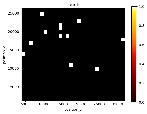
Visualization
lc.render_2d(dat, bin_size=1000, rescale=(0,100));
Analyze a localization property
We have a look at a certain localization property in locdata.
The analysis class LocalizationProperty provides a dataframe with the property as function of another property (index), and a plot or histogram of this property.
lprop = lc.LocalizationProperty(loc_property='intensity', index='frame')
lprop.compute(dat)
print(lprop.results.head())
       intensity
frame
0       33290.10
0       21275.40
0       20748.70
0        8531.77
0       14139.60
The plot shows results smoothed by a running average according to the specified window.
lprop.plot(window=100);
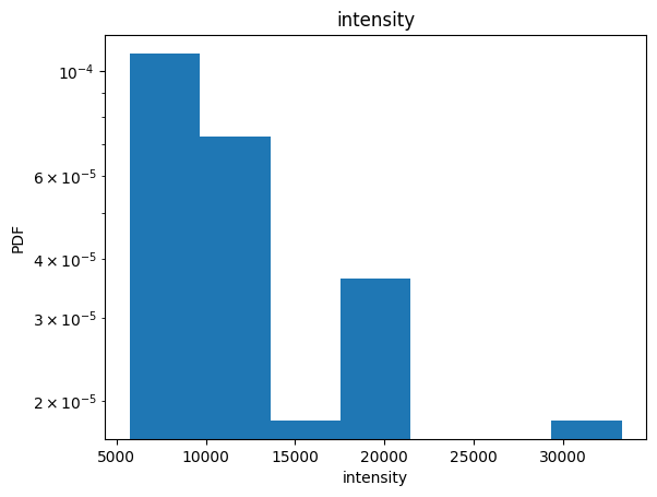
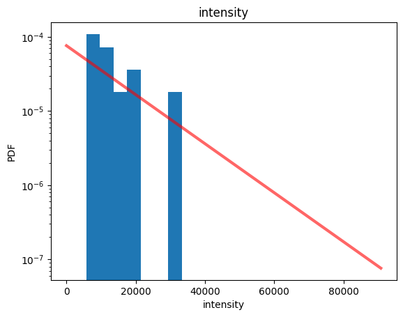
The histogram shows the probability density function of results.
lprop.hist(fit=False);
Per default the distribution is fitted to an exponential decay.
lprop.hist();
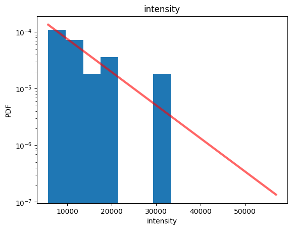
Fit results (as derived using the lmfit library) are provided in the distribution_statistics attribute.
lprop.distribution_statistics.parameter_dict()
{'intensity_loc': 5730.75, 'intensity_scale': 7411.226428571428}
lprop.results.min()
intensity    5730.75
dtype: float64
Fitting different distribution models
Per default the ‘with_constraints’ flag is True to apply standard fit constraints. This can be set to false and other parameters can be passed to the fit function.
lprop.fit_distributions(with_constraints=False, floc=0)
lprop.distribution_statistics.parameter_dict()
{'intensity_loc': 0.0, 'intensity_scale': 13141.976428571428}
lprop.hist(fit=True)
print(lprop.distribution_statistics.parameter_dict())
{'intensity_loc': 0.0, 'intensity_scale': 13141.976428571428}
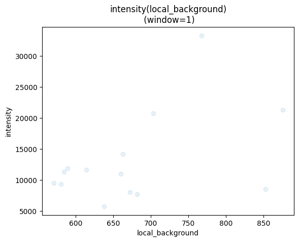
Showing correlations between two properties
By setting the index to another localization property correlations can be shown.
lprop = lc.LocalizationProperty(loc_property='intensity', index='local_background').compute(dat)
lprop.plot(marker='o', linestyle="", alpha=0.1);
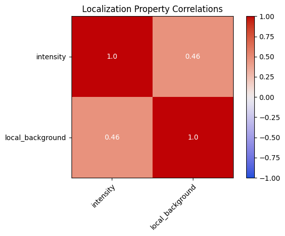
Correlation coefficients can be investigated in more detail using the LocalizationPropertyCorrelation class that is just a visualization of pandas.DataFrame.corr().
lpcorr = lc.LocalizationPropertyCorrelations(loc_properties=['intensity', 'local_background']).compute(dat)
lpcorr
LocalizationPropertyCorrelations(loc_properties=['intensity', 'local_background'])
lpcorr.plot();
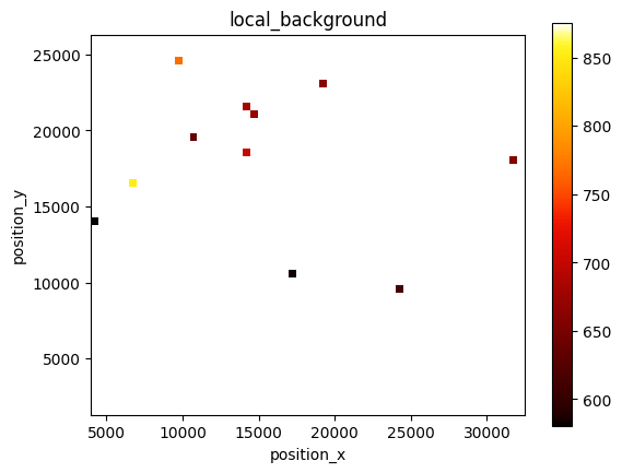
2-dimensional distribution of localization properties
In order to investigate a certain localization property in 2D you can just print the image with a color code representing the mean value of the chosen localization property in each bin.
lc.render_2d_mpl(dat, other_property='local_background', bin_size=500);
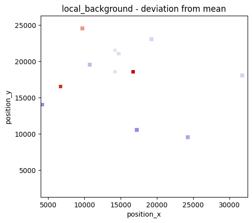
Otherwise use a specific class to analyse localization properties in 2d. Per default a bimodal normal distribution is fitted. This can e.g. help to check on even illumination during the recording.
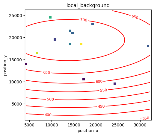
lprop2d = lc.LocalizationProperty2d(loc_properties=None, other_property='local_background', bin_size=500).compute(dat)
lprop2d.plot_deviation_from_mean();
lprop2d.plot(colors="r");
lprop2d.report()
Fit results for:

[[Model]]
    Model(model_function)
[[Fit Statistics]]
    # fitting method   = leastsq
    # function evals   = 43
    # data points      = 12
    # variables        = 5
    chi-square         = 75179.6882
    reduced chi-square = 10739.9555
    Akaike info crit   = 114.912757
    Bayesian info crit = 117.337290
    R-squared          = 0.25569453
[[Variables]]
    amplitude:  732.468389 +/- 47.0045236 (6.42%) (init = 875.461)
    center_x:   13822.4142 +/- 14800.9733 (107.08%) (init = 18245.59)
    center_y:   19401.6868 +/- 3825.17126 (19.72%) (init = 13803.61)
    sigma_x:    42169.8059 +/- 52664.9263 (124.89%) (init = 7125)
    sigma_y:    15484.6869 +/- 8624.45208 (55.70%) (init = 6250)
[[Correlations]] (unreported correlations are < 0.250)
    C(center_y, sigma_y)   = +0.7364
    C(center_x, sigma_x)   = -0.6514
    C(amplitude, sigma_y)  = -0.6030
    C(amplitude, sigma_x)  = -0.5552
    C(amplitude, center_y) = -0.4075
    C(center_y, sigma_x)   = +0.3845
    C(amplitude, center_x) = +0.3313
    C(sigma_x, sigma_y)    = +0.3140
    C(center_x, sigma_y)   = -0.2882
    C(center_x, center_y)  = -0.2544
Maximum fit value in image: 731.334
Minimum fit value in image: 580.351
Fit value variation over image range: 0.21