Tutorial about local density analysis

A local density is computed from the number of neighboring localizations within a specified radius.

from pathlib import Path

%matplotlib inline

import numpy as np
import matplotlib.pyplot as plt

import locan as lc

lc.show_versions(system=False, dependencies=False, verbose=False)

Locan:
   version: 0.22.0.dev32+g4bfc3ab8b

Python:
   version: 3.11.14

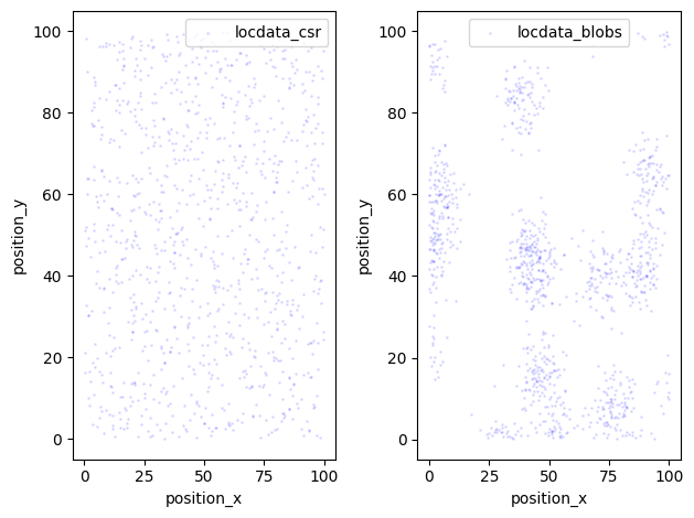
Synthetic data

We simulate localization data that is homogeneously Poisson distributed (also described as complete spatial randomness, csr).

rng = np.random.default_rng(seed=1)

locdata_csr = lc.simulate_Poisson(intensity=1e-1, region=((0,100), (0,100)), seed=rng)

print('Data head:')
print(locdata_csr.data.head(), '\n')
print('Summary:')
locdata_csr.print_summary()
print('Properties:')
print(locdata_csr.properties)

Jupyter environment detected. Enabling Open3D WebVisualizer.
[Open3D INFO] WebRTC GUI backend enabled.
[Open3D INFO] WebRTCWindowSystem: HTTP handshake server disabled.

Data head:
   position_x  position_y
0   14.415961   94.864945
1   31.183145   42.332645
2   82.770259   40.919914
3   54.959369    2.755911
4   75.351311   53.814331 

Summary:
identifier: "1"
comment: ""
source: SIMULATION
state: RAW
element_count: 1001
frame_count: 0
creation_time {
  2026-04-30T08:34:45.756356Z
}

Properties:
{'localization_count': 1001, 'position_x': np.float64(49.71480704304258), 'uncertainty_x': np.float64(0.8846806436903792), 'position_y': np.float64(50.34940144307567), 'uncertainty_y': np.float64(0.9309630174812346), 'region_measure_bb': np.float64(9970.499168748705), 'localization_density_bb': np.float64(0.10039617706779522), 'subregion_measure_bb': np.float64(399.40982202393604), 'region_measure': np.int64(10000), 'localization_density': np.float64(0.1001), 'subregion_measure': np.int64(400)}

We also simulate data that follows a Neyman-Scott distribution (blobs):

locdata_blob = lc.simulate_Thomas(parent_intensity=1e-3, region=((0, 100), (0, 100)), cluster_mu=100, cluster_std=5, seed=rng)

print('Data head:')
print(locdata_blob.data.head(), '\n')
print('Summary:')
locdata_blob.print_summary()
print('Properties:')
print(locdata_blob.properties)

Data head:
   position_x  position_y  cluster_label
0   74.134169    4.164725             25
1    1.755308   24.837606             20
2   38.929401   38.036252             28
3    1.465676   25.249268             20
4   74.866279   40.662736             18 

Summary:
identifier: "2"
comment: ""
source: SIMULATION
state: RAW
element_count: 1116
frame_count: 0
creation_time {
  2026-04-30T08:34:45.768812Z
}

Properties:
{'localization_count': 1116, 'position_x': np.float64(50.32464025249008), 'uncertainty_x': np.float64(0.8878228605015925), 'position_y': np.float64(41.51510460080934), 'uncertainty_y': np.float64(0.7620956001424609), 'region_measure_bb': np.float64(9969.531465793627), 'localization_density_bb': np.float64(0.11194106802602488), 'subregion_measure_bb': np.float64(399.3901705025785), 'region_measure': np.int64(10000), 'localization_density': np.float64(0.1116), 'subregion_measure': np.int64(400)}

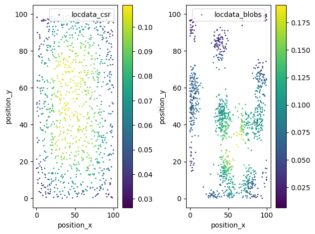
Scatter plot

fig, ax = plt.subplots(nrows=1, ncols=2)
locdata_csr.data.plot.scatter(x='position_x', y='position_y', ax=ax[0], color='Blue', s=1, alpha=0.1, label='locdata_csr')
locdata_blob.data.plot.scatter(x='position_x', y='position_y', ax=ax[1], color='Blue', s=1, alpha=0.1, label='locdata_blobs')
plt.tight_layout()
plt.show()

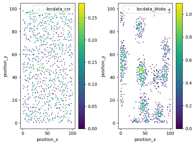
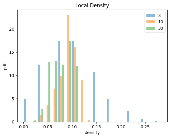
Local densities

We determine the local density for each localization and plot the probability density function for local densities.

lc.LocalDensity?

ld_csr = lc.LocalDensity(radii=[3, 10, 30])
ld_csr.compute(locdata_csr)
ld_csr.results.describe()

	3	10	30
count	1001.000000	1001.000000	1001.000000
mean	0.093348	0.090939	0.076425
std	0.054365	0.020611	0.020610
min	0.000000	0.019099	0.026526
25%	0.070736	0.079577	0.058357
50%	0.106103	0.095493	0.079224
75%	0.141471	0.105042	0.095139
max	0.282942	0.140056	0.108933

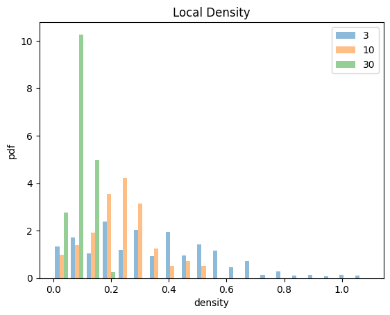
ld_blob = lc.LocalDensity(radii=[3, 10, 30])
ld_blob.compute(locdata_blob)
ld_blob.results.describe()

	3	10	30
count	1116.000000	1116.000000	1116.000000
mean	0.345628	0.237877	0.089437
std	0.222333	0.111080	0.035233
min	0.000000	0.000000	0.006720
25%	0.176839	0.168704	0.064723
50%	0.318310	0.232366	0.094078
75%	0.495149	0.299211	0.113884
max	1.096401	0.547493	0.190986

radius = 3
fig, ax = plt.subplots(nrows=1, ncols=2)
locdata_csr.data.plot.scatter(x='position_x', y='position_y', ax=ax[0], color=ld_csr.results[radius], s=1, colormap='viridis', alpha=1, label='locdata_csr')
locdata_blob.data.plot.scatter(x='position_x', y='position_y', ax=ax[1], color=ld_blob.results[radius], s=1, colormap='viridis', alpha=1, label='locdata_blobs')
plt.tight_layout()
plt.show()

/tmp/ipykernel_877/23467711.py:3: UserWarning: 'color' and 'colormap' cannot be used simultaneously. Using 'color'
  locdata_csr.data.plot.scatter(x='position_x', y='position_y', ax=ax[0], color=ld_csr.results[radius], s=1, colormap='viridis', alpha=1, label='locdata_csr')
/tmp/ipykernel_877/23467711.py:4: UserWarning: 'color' and 'colormap' cannot be used simultaneously. Using 'color'
  locdata_blob.data.plot.scatter(x='position_x', y='position_y', ax=ax[1], color=ld_blob.results[radius], s=1, colormap='viridis', alpha=1, label='locdata_blobs')

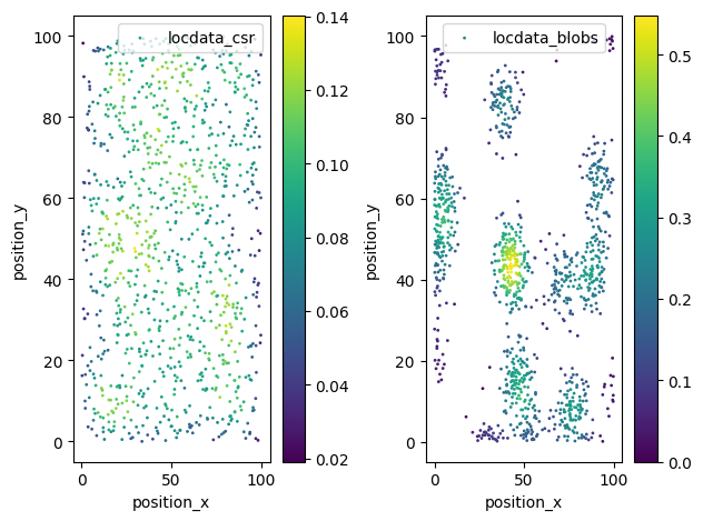
radius = 10
fig, ax = plt.subplots(nrows=1, ncols=2)
locdata_csr.data.plot.scatter(x='position_x', y='position_y', ax=ax[0], color=ld_csr.results[radius], s=1, colormap='viridis', alpha=1, label='locdata_csr')
locdata_blob.data.plot.scatter(x='position_x', y='position_y', ax=ax[1], color=ld_blob.results[radius], s=1, colormap='viridis', alpha=1, label='locdata_blobs')
plt.tight_layout()
plt.show()

/tmp/ipykernel_877/3710508265.py:3: UserWarning: 'color' and 'colormap' cannot be used simultaneously. Using 'color'
  locdata_csr.data.plot.scatter(x='position_x', y='position_y', ax=ax[0], color=ld_csr.results[radius], s=1, colormap='viridis', alpha=1, label='locdata_csr')

/tmp/ipykernel_877/3710508265.py:4: UserWarning: 'color' and 'colormap' cannot be used simultaneously. Using 'color'
  locdata_blob.data.plot.scatter(x='position_x', y='position_y', ax=ax[1], color=ld_blob.results[radius], s=1, colormap='viridis', alpha=1, label='locdata_blobs')

radius = 30
fig, ax = plt.subplots(nrows=1, ncols=2)
locdata_csr.data.plot.scatter(x='position_x', y='position_y', ax=ax[0], color=ld_csr.results[radius], s=1, colormap='viridis', alpha=1, label='locdata_csr')
locdata_blob.data.plot.scatter(x='position_x', y='position_y', ax=ax[1], color=ld_blob.results[radius], s=1, colormap='viridis', alpha=1, label='locdata_blobs')
plt.tight_layout()
plt.show()

/tmp/ipykernel_877/1649477093.py:3: UserWarning: 'color' and 'colormap' cannot be used simultaneously. Using 'color'
  locdata_csr.data.plot.scatter(x='position_x', y='position_y', ax=ax[0], color=ld_csr.results[radius], s=1, colormap='viridis', alpha=1, label='locdata_csr')

/tmp/ipykernel_877/1649477093.py:4: UserWarning: 'color' and 'colormap' cannot be used simultaneously. Using 'color'
  locdata_blob.data.plot.scatter(x='position_x', y='position_y', ax=ax[1], color=ld_blob.results[radius], s=1, colormap='viridis', alpha=1, label='locdata_blobs')

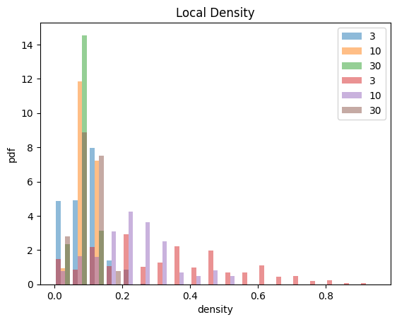
ld_csr.hist(alpha=0.5, density=True, bins=20);

ld_blob.hist(alpha=0.5, density=True, bins=20);

bins = np.arange(0, 1, 0.05)
ld_csr.hist(alpha=0.5, bins=bins)
ld_blob.hist(alpha=0.5, bins=bins);

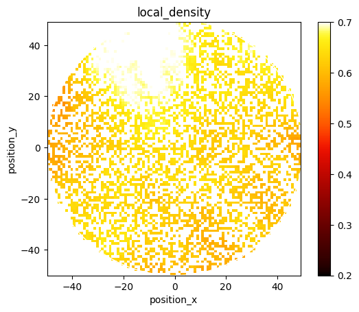
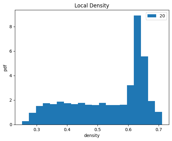
Local densities with boundary correction

We determine the local density for each localization with a boundary correction applied. For the correction local density values are normalized by the relative overlapp of the encircling region and the support region.

locdata = lc.simulate_uniform(n_samples=5_000, region=lc.Ellipse((0, 0), 100, 100))
locdata.region

radius = 20

ld = lc.LocalDensity(radii=[radius]).compute(locdata)

ld.hist(bins=20);

ld.results.index = locdata.data.index
df = locdata.dataframe.assign(local_density=ld.results[radius])
locdata = locdata.update(dataframe=df)
locdata.data.local_density.describe()

count    5000.000000
mean        0.533202
std         0.121798
min         0.252261
25%         0.427331
50%         0.580120
75%         0.635824
max         0.710627
Name: local_density, dtype: float64

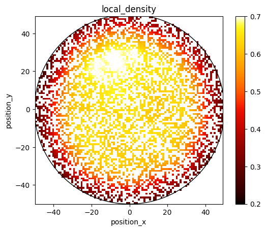
fig, ax = plt.subplots()
lc.render_2d_mpl(locdata, ax=ax, loc_properties=["position_x", "position_y"], bin_size=1, other_property='local_density', rescale=lc.Trafo.NONE, vmin=0.2, vmax=0.7);
if locdata.region:
    locdata.region.plot(ax=ax, fill=False, color='Black');

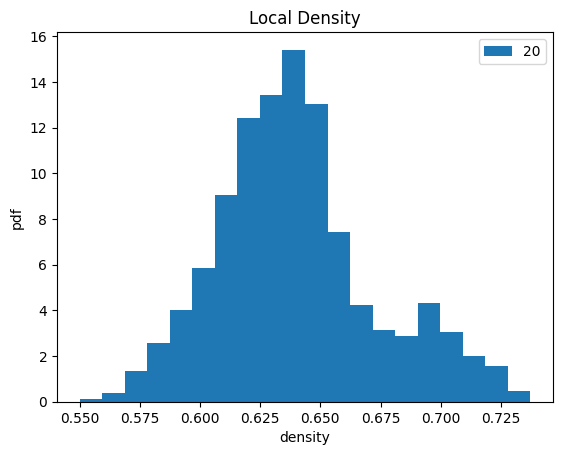
ld_2 = lc.LocalDensity(radii=[radius], boundary_correction=True).compute(locdata)

ld_2.hist(bins=20);

ld_2.results.index = locdata.data.index
df = locdata.dataframe.assign(local_density=ld_2.results[radius])
locdata = locdata.update(dataframe=df)
locdata.data.local_density.describe()

count    5000.000000
mean        0.639977
std         0.033068
min         0.549939
25%         0.618943
50%         0.636847
75%         0.655578
max         0.737318
Name: local_density, dtype: float64

fig, ax = plt.subplots()
lc.render_2d_mpl(locdata, ax=ax, loc_properties=["position_x", "position_y"], bin_size=1, other_property='local_density', rescale=lc.Trafo.NONE, vmin=0.2, vmax=0.7);
if locdata.region:
    locdata.region.plot(ax=ax, fill=False, color='White');