Tutorial about localization precision

Localization precision is determined from consecutive localizations that are identified within a certain search radius. The results include the distances between localization pairs, the position deltas for each coordinate and the corresponding frame of the first localizations.

from pathlib import Path

%matplotlib inline

import matplotlib.pyplot as plt

import locan as lc

lc.show_versions(system=False, dependencies=False, verbose=False)

Locan:
   version: 0.22.0.dev32+g4bfc3ab8b

Python:
   version: 3.11.14

# A path in which test data can be found:
TEST_DIR: Path = Path.cwd().parents[2] / "tests"
TEST_DIR

PosixPath('/home/docs/checkouts/readthedocs.org/user_builds/locan/checkouts/latest/tests')

Load SMLM data file

Identify some data in the test_data directory and provide a path using pathlib.Path (returned by lc.ROOT_DIR)

path = TEST_DIR / 'test_data/npc_gp210.asdf'
print(path, '\n')
dat = lc.load_locdata(path=path, file_type=lc.FileType.ASDF)

/home/docs/checkouts/readthedocs.org/user_builds/locan/checkouts/latest/tests/test_data/npc_gp210.asdf 

Jupyter environment detected. Enabling Open3D WebVisualizer.
[Open3D INFO] WebRTC GUI backend enabled.
[Open3D INFO] WebRTCWindowSystem: HTTP handshake server disabled.

Print information about the data:

print(dat.data.head(), '\n')
print('Summary:')
dat.print_summary()
print('Properties:')
print(dat.properties)

    position_x   position_y  frame     intensity  two_kernel_improvement  \
0  5631.709961  6555.850098     24  21800.699219                     0.0   
1  5642.899902  6550.990234     25  23352.900391                     0.0   
2  5610.319824  6546.819824     26   5007.509766                     0.0   
3  5713.299805  6611.950195    141   6437.140137                     0.0   
4  5699.750000  6627.390137    142  19998.300781                     0.0   

   chi_square  local_background  
0   1426930.0       1188.489990  
1    983634.0       1135.199951  
2    577707.0       1107.219971  
3    616255.0       1118.430054  
4    903412.0       1144.709961   

Summary:
identifier: "5"
comment: ""
source: EXPERIMENT
state: MODIFIED
element_count: 202
frame_count: 202
file {
  type: ASDF
  path: "/home/docs/checkouts/readthedocs.org/user_builds/locan/checkouts/latest/tests/test_data/npc_gp210.asdf"
}
creation_time {
  2024-01-23T08:32:31.518779Z
}
modification_time {
  2024-01-23T08:32:31.518779Z
}

Properties:
{'localization_count': 202, 'position_x': np.float64(5623.488892810179), 'uncertainty_x': np.float64(3.9700846636030356), 'position_y': np.float64(6625.534602703435), 'uncertainty_y': np.float64(3.999303432482808), 'intensity': np.float32(3944778.0), 'local_background': np.float32(1131.3207), 'frame': np.int16(24), 'region_measure_bb': np.float32(47134.543), 'localization_density_bb': np.float32(0.004285604), 'subregion_measure_bb': np.float32(870.98047)}

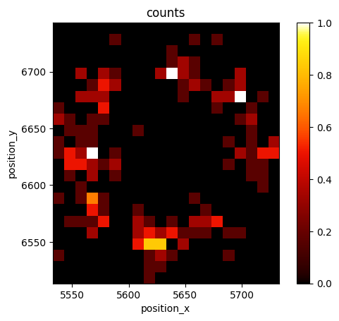
Visualization

lc.render_2d(dat, bin_size=10, rescale=(0,100));

Analyze localization precision

lp = lc.LocalizationPrecision(radius=50)

lp.compute(dat)
lp.results.head()

Processed frames::   0%|          | 0/24884 [00:00<?, ?it/s]

Processed frames::   8%|▊         | 2096/24884 [00:00<00:01, 20958.67it/s]

Processed frames::  25%|██▍       | 6149/24884 [00:00<00:00, 32467.70it/s]

Processed frames::  46%|████▌     | 11338/24884 [00:00<00:00, 40818.35it/s]

Processed frames:: 100%|██████████| 24884/24884 [00:00<00:00, 62478.86it/s]

	position_delta_x	position_delta_y	position_distance	original_index	frame
0	-11.189941	4.859863	12.199716	0	24
1	32.580078	4.170410	32.845909	1	25
2	13.549805	-15.439941	20.542370	3	141
3	4.669922	3.010254	5.556060	4	142
4	20.469727	14.750000	25.230383	6	239

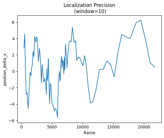
The plot

lp.plot(loc_property='position_delta_x', window=10);

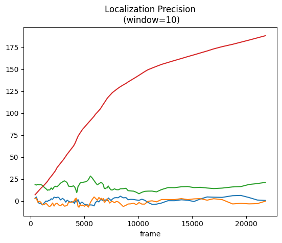
lp.plot(window=10);

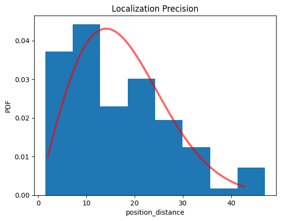
The histogram for the distances per default includes a fit to a distribution expected for normal distributed localizations. Sigma / sqrt(2) is the localization precision.

lp.hist();

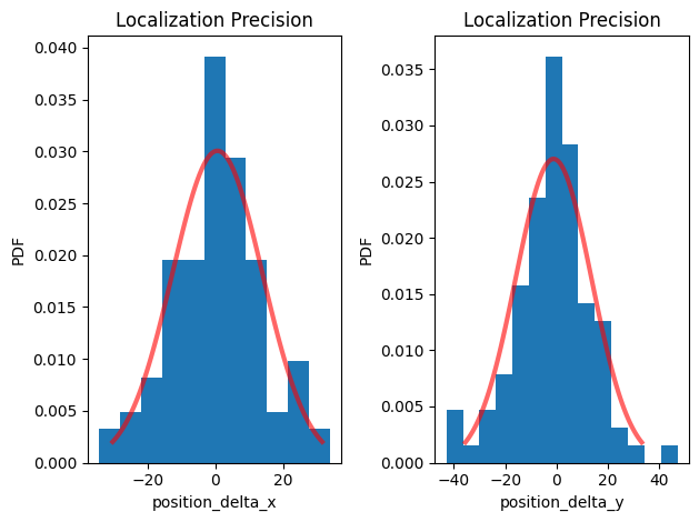
Alternatively the position deltas can be histogrammed.

fig, ax = plt.subplots(nrows=1, ncols=2)
lp.hist(ax=ax[0], loc_property='position_delta_x')
lp.hist(ax=ax[1], loc_property='position_delta_y')
plt.tight_layout()
plt.show()

Fit distributions and show parameters

Appropriate distribution functions are fitted to the data either by calling the hist function or by running:

lp.fit_distributions()

The estimated fit parameters are provided under the distribution_statistics attribute

lp.distribution_statistics.parameter_dict()

{'position_delta_x_loc': np.float32(0.6029139),
 'position_delta_x_scale': np.float32(13.2682),
 'position_delta_y_loc': np.float32(-1.227687),
 'position_delta_y_scale': np.float32(14.76087),
 'position_distance_sigma': np.float64(14.067675781250028),
 'position_distance_loc': 0,
 'position_distance_scale': 1}

Remember: localization precision is typically defined as the standard deviation for the distances between localizations and their center position (the true dye position). Therefore, the estimated sigmas have to be divided by sqrt(2) to yield localization precision.