Tutorial about clustering localizations data

Locan provides methods for clustering localizations in LocData objects. The methods all return a new LocDat object that represents the collected selections for each cluster.

from pathlib import Path

%matplotlib inline

import numpy as np
import pandas as pd
import matplotlib.pyplot as plt
from mpl_toolkits.mplot3d import Axes3D

import locan as lc

/tmp/ipykernel_1299/1692805095.py:6: DeprecationWarning: 
Pyarrow will become a required dependency of pandas in the next major release of pandas (pandas 3.0),
(to allow more performant data types, such as the Arrow string type, and better interoperability with other libraries)
but was not found to be installed on your system.
If this would cause problems for you,
please provide us feedback at https://github.com/pandas-dev/pandas/issues/54466
        
  import pandas as pd

lc.show_versions(system=False, dependencies=False, verbose=False)

Locan:
   version: 0.20.0.dev41+g755b969

Python:
   version: 3.11.6

Synthetic data

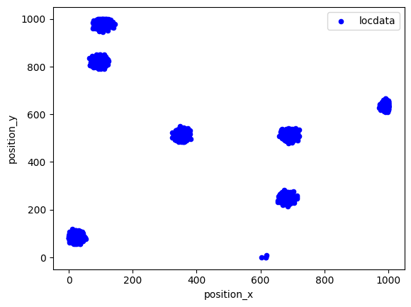
We simulate localization data that follows a Neyman-Scott distribution in 2D:

rng = np.random.default_rng(seed=11)

locdata = lc.simulate_Thomas(parent_intensity=1e-5, region=((0, 1000), (0, 1000)), cluster_mu=1000, cluster_std=10, seed=rng)

locdata.print_summary()

Jupyter environment detected. Enabling Open3D WebVisualizer.
[Open3D INFO] WebRTC GUI backend enabled.
[Open3D INFO] WebRTCWindowSystem: HTTP handshake server disabled.
identifier: "1"
comment: ""
source: SIMULATION
state: RAW
element_count: 6409
frame_count: 0
creation_time {
  2024-03-14T11:08:06.174673Z
}

fig, ax = plt.subplots(nrows=1, ncols=1)
locdata.data.plot.scatter(x='position_x', y='position_y', ax=ax, color='Blue', label='locdata')
plt.show()

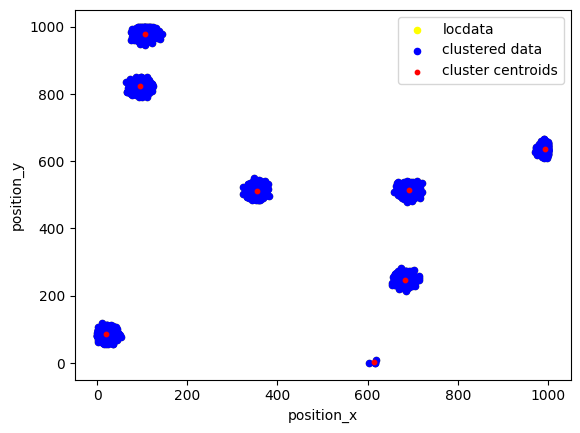
Cluster localizations by dbscan

noise, clust = lc.cluster_dbscan(locdata, eps=20, min_samples=3)
assert noise.data.empty

fig, ax = plt.subplots(nrows=1, ncols=1)
locdata.data.plot.scatter(x='position_x', y='position_y', ax=ax, color='Yellow', label='locdata')
lc.LocData.concat(clust.references).data.plot.scatter(x='position_x', y='position_y', ax=ax, color='Blue', label='clustered data')
clust.data.plot.scatter(x='position_x', y='position_y', ax=ax, color='Red', s=10, label='cluster centroids')
plt.show()

clust.data.head()

	localization_count	position_x	uncertainty_x	position_y	uncertainty_y	region_measure_bb	localization_density_bb	subregion_measure_bb	region_measure	localization_density	subregion_measure
0	1016	20.379759	0.300643	85.374381	0.314089	3262.794976	0.311389	229.091796	1000000	0.001016	4000
1	1050	681.909709	0.305784	248.276785	0.310572	4122.205751	0.254718	257.346576	1000000	0.001050	4000
2	986	353.614004	0.302981	512.621728	0.320747	3814.439353	0.258491	248.125971	1000000	0.000986	4000
3	996	690.951712	0.315008	513.619337	0.313548	3935.485208	0.253082	250.933843	1000000	0.000996	4000
4	368	992.523811	0.288485	636.239028	0.548494	1650.773324	0.222926	170.375014	1000000	0.000368	4000

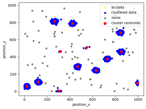
Cluster localizations in the presence of noise

Often homogeneously distributed localizations are present that cannot be clustered (so-called noise). In this case noise should be set True such that two LocData objects are returned that hold noise and the cluster collection. If noise is False it will be part of the returned cluster collection.

locdata_cluster = lc.simulate_Thomas(parent_intensity=1e-5, region=((0, 1000), (0, 1000)), cluster_mu=1000, cluster_std=10, seed=rng)
locdata_noise = lc.simulate_Poisson(intensity=1e-4, region=((0, 1000), (0, 1000)), seed=rng)
locdata = lc.LocData.concat([locdata_cluster, locdata_noise])

noise, clust = lc.cluster_dbscan(locdata, eps=30, min_samples=3)

fig, ax = plt.subplots(nrows=1, ncols=1)
locdata.data.plot.scatter(x='position_x', y='position_y', ax=ax, color='Yellow', label='locdata')
lc.LocData.concat(clust.references).data.plot.scatter(x='position_x', y='position_y', ax=ax, color='Blue', label='clustered data')
noise.data.plot.scatter(x='position_x', y='position_y', ax=ax, color='Gray', label='noise')
clust.data.plot.scatter(x='position_x', y='position_y', ax=ax, color='Red', s=50, label='cluster centroids')
plt.show()

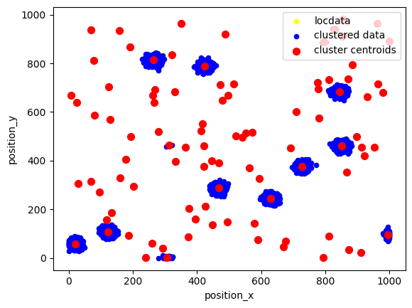
If single localizations should be inlcuded as individual clusters, we need to reduce min_samples to 1. In that case noise will always be None.

noise, clust = lc.cluster_dbscan(locdata, eps=20, min_samples=1)
assert noise.data.empty

fig, ax = plt.subplots(nrows=1, ncols=1)
locdata.data.plot.scatter(x='position_x', y='position_y', ax=ax, color='Yellow', label='locdata')
lc.LocData.concat(clust.references).data.plot.scatter(x='position_x', y='position_y', ax=ax, color='Blue', label='clustered data')
# noise.data.plot.scatter(x='position_x', y='position_y', ax=ax, color='Gray', label='noise')
clust.data.plot.scatter(x='position_x', y='position_y', ax=ax, color='Red', s=50, label='cluster centroids')
plt.show()

Other cluster functions are available in the locan.data.clustermodule.