Tutorial about regions

Regions define a support for localization data or specify a hull that captures a set of localizations. Locan provides various region classes with a standard set of attributes and methods.

%matplotlib inline

import numpy as np
import pandas as pd
import matplotlib.pyplot as plt

import locan as lc

/tmp/ipykernel_1910/3049569888.py:4: DeprecationWarning: 
Pyarrow will become a required dependency of pandas in the next major release of pandas (pandas 3.0),
(to allow more performant data types, such as the Arrow string type, and better interoperability with other libraries)
but was not found to be installed on your system.
If this would cause problems for you,
please provide us feedback at https://github.com/pandas-dev/pandas/issues/54466
        
  import pandas as pd

lc.show_versions(system=False, dependencies=False, verbose=False)

Locan:
   version: 0.20.0.dev41+g755b969

Python:
   version: 3.11.6

Region definitions

The standard set of attributes and methods is defined by the abstract base class Region that all region classes inherit.

lc.Region?

Jupyter environment detected. Enabling Open3D WebVisualizer.
[Open3D INFO] WebRTC GUI backend enabled.
[Open3D INFO] WebRTCWindowSystem: HTTP handshake server disabled.

print("Methods:")
[method for method in dir(lc.Region) if not method.startswith('_')]

Methods:

['bounding_box',
 'bounds',
 'buffer',
 'centroid',
 'contains',
 'dimension',
 'extent',
 'from_intervals',
 'intersection',
 'max_distance',
 'points',
 'region_measure',
 'subregion_measure',
 'symmetric_difference',
 'union']

Further definitions can be found in the abstract classes Region1D, Region2D and Region3D and all specific region classes.

import inspect
inspect.getmembers(lc.data.region, inspect.isabstract)

[('Region', locan.data.region.Region),
 ('Region1D', locan.data.region.Region1D),
 ('Region2D', locan.data.region.Region2D),
 ('Region3D', locan.data.region.Region3D),
 ('RegionND', locan.data.region.RegionND)]

Use Region classes

Use one of the following classes to define a region in 1, 2 or 3 dimensions:

print("Empty Region:\n", [lc.EmptyRegion.__name__], "\n")
print("Regions in 1D:\n", [cls.__name__ for cls in lc.Region1D.__subclasses__()], "\n")
print("Regions in 2D:\n", [cls.__name__ for cls in lc.Region2D.__subclasses__()], "\n")
print("Regions in 3D:\n", [cls.__name__ for cls in lc.Region3D.__subclasses__()], "\n")
print("Regions in nD:\n", [cls.__name__ for cls in lc.RegionND.__subclasses__()], "\n")

Empty Region:
 ['EmptyRegion'] 

Regions in 1D:
 ['Interval'] 

Regions in 2D:
 ['Rectangle', 'Ellipse', 'Polygon', 'MultiPolygon'] 

Regions in 3D:
 ['AxisOrientedCuboid', 'Cuboid'] 

Regions in nD:
 ['AxisOrientedHypercuboid'] 

The region constructors take different parameters.

REMEMBER: Angles are taken in degrees.

region = lc.Rectangle(corner=(0, 0), width=1, height=2, angle=45)
region

points = ((0, 0), (0, 1), (1, 1), (1, 0.5), (0, 0))
holes = [((0.2, 0.2), (0.2, 0.4), (0.4, 0.4), (0.3, 0.25)), ((0.5, 0.5), (0.5, 0.8), (0.8, 0.8), (0.7, 0.45))]
region = lc.Polygon(points, holes)
print(region)
region

Polygon(<self.points>, <self.holes>)

Several attributes are available, e.g. about the area or circumference.

dict(dimension=region.dimension, bounds=region.bounds, extent=region.extent, bounding_box=region.bounding_box, centroid=region.centroid, max_distance=region.max_distance, 
     region_measure= region.region_measure, subregion_measure=region.subregion_measure)  

{'dimension': 2,
 'bounds': array([0., 0., 1., 1.]),
 'extent': array([1., 1.]),
 'bounding_box': Rectangle((0.0, 0.0), 1.0, 1.0, 0),
 'centroid': array([0.42723735, 0.61770428]),
 'max_distance': 1.4142135623730951,
 'region_measure': 0.6425,
 'subregion_measure': 5.480275727142994}

A list of points defining a polygon that resembles the region is available.

print("Points:\n", region.points, "\n")
print("Holes:\n", region.holes)

Points:
 [[0.  0. ]
 [0.  1. ]
 [1.  1. ]
 [1.  0.5]
 [0.  0. ]] 

Holes:
 [array([[0.2 , 0.2 ],
       [0.2 , 0.4 ],
       [0.4 , 0.4 ],
       [0.3 , 0.25]]), array([[0.5 , 0.5 ],
       [0.5 , 0.8 ],
       [0.8 , 0.8 ],
       [0.7 , 0.45]])]

Region can be constructed from interval tuples indicating feature ranges.

region_1d = lc.Region.from_intervals((0, 1))
region_2d = lc.Region.from_intervals(((0, 1), (0, 1)))
region_3d = lc.Region.from_intervals([(0, 1)] * 3)
region_4d = lc.Region.from_intervals([(0, 1)] * 4)

for region in (region_1d, region_2d, region_3d, region_4d):
    print(region)

Interval(0, 1)
Rectangle((0, 0), 1, 1, 0)
AxisOrientedCuboid((0, 0, 0), 1, 1, 1)
AxisOrientedHypercuboid((0, 0, 0, 0), (1, 1, 1, 1))

Plot regions

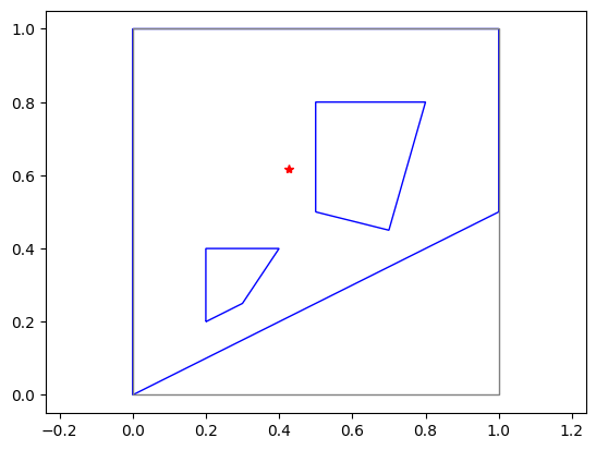
Regions can be plotted as patch in mathplotlib figures.

points = ((0, 0), (0, 1), (1, 1), (1, 0.5), (0, 0))
holes = [((0.2, 0.2), (0.2, 0.4), (0.4, 0.4), (0.3, 0.25)), ((0.5, 0.5), (0.5, 0.8), (0.8, 0.8), (0.7, 0.45))]
region = lc.Polygon(points, holes)

fig, ax = plt.subplots(nrows=1, ncols=1)
ax.add_patch(region.as_artist(fill=False, color='Blue'))
ax.add_patch(region.bounding_box.as_artist(fill=False, color='Grey'))
ax.plot(*region.centroid, '*', color='Red')
ax.axis('equal')
plt.show()

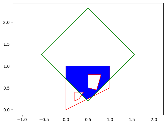
Intersection, union, difference of regions

Methods are provided to check for intersection, difference, union and membership.

other_region = lc.Rectangle(corner=(0.5, 0.2), width=1.5, height=1.5, angle=45)
other_region.shapely_object

result = region.intersection(other_region)
print(result)

Polygon(<self.points>, <self.holes>)

fig, ax = plt.subplots(nrows=1, ncols=1)
ax.add_patch(result.as_artist(fill=True, color='Blue'))
ax.add_patch(region.as_artist(fill=False, color='Red'))
ax.add_patch(other_region.as_artist(fill=False, color='Green'))
ax.axis('equal')
plt.show()

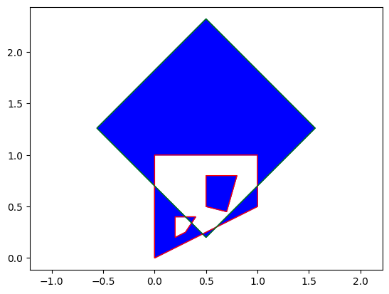
result = region.symmetric_difference(other_region)
print(result)

MultiPolygon(<self.polygons>)

fig, ax = plt.subplots(nrows=1, ncols=1)
ax.add_patch(result.as_artist(fill=True, color='Blue'))
ax.add_patch(region.as_artist(fill=False, color='Red'))
ax.add_patch(other_region.as_artist(fill=False, color='Green'))
ax.axis('equal')
plt.show()

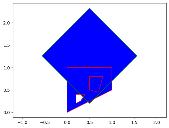
result = region.union(other_region)
print(result)

Polygon(<self.points>, <self.holes>)

fig, ax = plt.subplots(nrows=1, ncols=1)
ax.add_patch(result.as_artist(fill=True, color='Blue'))
ax.add_patch(region.as_artist(fill=False, color='Red'))
ax.add_patch(other_region.as_artist(fill=False, color='Green'))
ax.axis('equal')
plt.show()

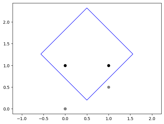
Check if point is in region

Region has a contains method to select points that are within the region.

inside_indices = other_region.contains(region.points)
contained_points = region.points[inside_indices]

fig, ax = plt.subplots(nrows=1, ncols=1)
ax.scatter(*region.points.T, color='Grey')
ax.scatter(*contained_points.T, color='Black')
ax.add_patch(other_region.as_artist(fill=False, color='Blue'))
ax.axis('equal')
plt.show()

LocData and regions

LocData bring various hulls that define regions. Also LocData typically has a unique region defined as support. This can e.g. result from the definition of a region of interest using the ROI function or as specified in a corresponding yaml file.

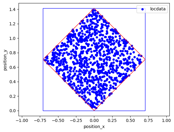
Create data in region:

A random dataset is created within a specified region (for other methods see simulation tutorial).

region = lc.Rectangle(corner=(0, 0), width=1, height=1, angle=45)
locdata = lc.simulate_uniform(n_samples=1000, region=region, seed=1)
locdata.print_summary()

identifier: "1"
comment: ""
source: SIMULATION
state: RAW
element_count: 1000
frame_count: 0
creation_time {
  2024-03-14T11:09:42.437524Z
}

region

Show scatter plots together with regions

fig, ax = plt.subplots(nrows=1, ncols=1)
locdata.data.plot.scatter(x='position_x', y='position_y', ax=ax, color='Blue', label='locdata')
ax.add_patch(locdata.region.as_artist(fill=False, color='Red'))
ax.add_patch(locdata.region.bounding_box.as_artist(fill=False, color='Blue'))
ax.axis('equal')
plt.show()

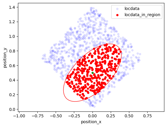
Select localizations within regions

LocData can be selected for localizations being inside the region.

region = lc.Ellipse(center=(0, 0.5), width=1, height=0.5, angle=45)
locdata_in_region = lc.select_by_region(locdata, region)
locdata_in_region.region

fig, ax = plt.subplots(nrows=1, ncols=1)
locdata.data.plot.scatter(x='position_x', y='position_y', ax=ax, color='Blue', label='locdata', alpha=0.1)
ax.add_patch(region.as_artist(fill=False, color='Red'))
locdata_in_region.data.plot.scatter(x='position_x', y='position_y', ax=ax, color='Red', label='locdata_in_region')
ax.plot(*region.centroid, '*', color='Green')
ax.axis('equal')
plt.show()

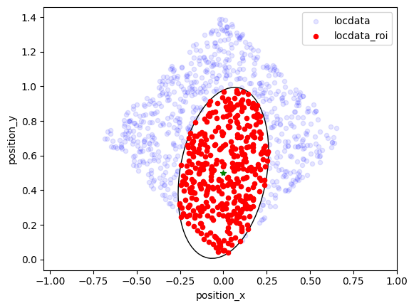
Regions of interest

The Roi class is an object that defines a region of interest for a specific localization dataset. It is mostly used to save and reload regions of interest after having selected them interactively, e.g. in napari. It is therefore related to region specifications and a unique LocData object.

Define a region of interest (roi):

roi = lc.Roi(reference=locdata, region=lc.Ellipse(center=(0, 0.5), width=1, height=0.5, angle=80))
roi

Roi(reference=<locan.data.locdata.LocData object at 0x7f9c41de7550>, region=Ellipse((0.0, 0.5), 1, 0.5, 80),  loc_properties=())

Create new LocData instance by selecting localizations within a roi.

locdata_roi = roi.locdata()

fig, ax = plt.subplots(nrows=1, ncols=1)
locdata.data.plot.scatter(x='position_x', y='position_y', ax=ax, color='Blue', label='locdata', alpha=0.1)
ax.add_patch(roi.region.as_artist(fill=False))
locdata_roi.data.plot.scatter(x='position_x', y='position_y', ax=ax, color='Red', label='locdata_roi')
ax.plot(*roi.region.centroid, '*', color='Green')
ax.axis('equal')
plt.show()

ROI input/output

If you have prepared rois and saved them as roi.yaml file you can read that data back in:

import tempfile
from pathlib import Path

with tempfile.TemporaryDirectory() as tmp_directory:
    file_path = Path(tmp_directory) / 'roi.yaml'

    roi.to_yaml(path=file_path)

    roi_new = lc.Roi.from_yaml(path = file_path)
    roi_new.reference = roi.reference
    
new_locdata = roi_new.locdata()
new_locdata.meta

/home/docs/checkouts/readthedocs.org/user_builds/locan/envs/latest/lib/python3.11/site-packages/locan/rois/roi.py:300: UserWarning: The localization data has to be saved and the file path provided, or the reference is lost.
  warnings.warn(

identifier: "4"
source: SIMULATION
state: MODIFIED
history {
  name: "make_uniform"
  parameter: "{\'n_samples\': 1000, \'region\': Rectangle((0, 0), 1, 1, 45), \'seed\': 1}"
}
history {
  name: "locdata"
  parameter: "{\'self\': Roi(reference=<locan.data.locdata.LocData object at 0x7f9c41de7550>, region=Ellipse((0.0, 0.5), 1, 0.5, 80),  loc_properties=[]), \'reduce\': True}"
}
ancestor_identifiers: "1"
element_count: 388
frame_count: 0
creation_time {
  seconds: 1710414582
  nanos: 437524000
}
modification_time {
  seconds: 1710414582
  nanos: 437524000
}

roi_new

Roi(reference=<locan.data.locdata.LocData object at 0x7f9c41de7550>, region=Ellipse((0.0, 0.5), 1, 0.5, 80),  loc_properties=[])