Tutorial about mutiprocessing using ray

We will describe how to set up an analysis pipeline to process multiple datasets in parallel using the framework ray.

import sys
import logging

%matplotlib inline

import numpy as np
import pandas as pd
import matplotlib.pyplot as plt
import ray

import locan as lc

/tmp/ipykernel_1620/3782818269.py:7: DeprecationWarning: 
Pyarrow will become a required dependency of pandas in the next major release of pandas (pandas 3.0),
(to allow more performant data types, such as the Arrow string type, and better interoperability with other libraries)
but was not found to be installed on your system.
If this would cause problems for you,
please provide us feedback at https://github.com/pandas-dev/pandas/issues/54466
        
  import pandas as pd

lc.show_versions(dependencies=False, verbose=False)

Locan:
   version: 0.20.0.dev41+g755b969

Python:
   version: 3.11.6

System:
python-bits: 64
    system: Linux
   release: 5.19.0-1028-aws
   version: #29~22.04.1-Ubuntu SMP Tue Jun 20 19:12:11 UTC 2023
   machine: x86_64
 processor: x86_64
 byteorder: little
    LC_ALL: None
      LANG: C.UTF-8
    LOCALE: {'language-code': 'en_US', 'encoding': 'UTF-8'}

Activate logging

logging.basicConfig(stream=sys.stdout, level=logging.INFO, format='%(asctime)s - %(name)s - %(levelname)s - %(message)s')
logger = logging.getLogger()

For changing the configuration logging has to be reloaded or the kernel be restarted.

Synthetic data

Simulate 3 datasets of localization data that is homogeneously Poisson distributed and treat them as files.

rng = np.random.default_rng(seed=1)

locdatas = [lc.simulate_Poisson(intensity=1e-3, region=((0,1000), (0,1000)), seed=rng) for _ in range(3)]
files = locdatas

print("Element_counts:", [locdata.meta.element_count for locdata in locdatas])

Jupyter environment detected. Enabling Open3D WebVisualizer.
[Open3D INFO] WebRTC GUI backend enabled.
[Open3D INFO] WebRTCWindowSystem: HTTP handshake server disabled.
Element_counts: [1001, 994, 978]

Analysis pipeline

Define an analysis pipeline. Typically a pipeline processes a single file, which in this example will be a an element of locdatas.

Within the analysis procedure there will be more random number generation involved. Therefore a correctly generated seed has to be passed.

def computation(self, file, seed):
    logging.basicConfig(level=logging.INFO)
    logger.info(f'computation started for file: {file}')
    
    rng = np.random.default_rng(seed=seed)
    
    other_locdata = lc.simulate_Poisson(intensity=1e-3, region=((0,1000), (0,1000)), seed=rng)
    self.nn = lc.NearestNeighborDistances().compute(locdata=file, other_locdata=other_locdata)
        
    return self

Run analysis in parallel

ray.init()
# ray.init(num_cpus = 4)

2024-03-14 11:09:23,446	WARNING services.py:1996 -- WARNING: The object store is using /tmp instead of /dev/shm because /dev/shm has only 67108864 bytes available. This will harm performance! You may be able to free up space by deleting files in /dev/shm. If you are inside a Docker container, you can increase /dev/shm size by passing '--shm-size=1.76gb' to 'docker run' (or add it to the run_options list in a Ray cluster config). Make sure to set this to more than 30% of available RAM.

2024-03-14 11:09:24,601	INFO worker.py:1715 -- Started a local Ray instance. View the dashboard at http://127.0.0.1:8265 

%%time
@ray.remote
def worker(file, seed):
    pipe = lc.Pipeline(computation=computation, file=file, seed=seed).compute()
    return pipe

n_processes = len(files)
ss = np.random.SeedSequence()
child_seeds = ss.spawn(n_processes)

futures = [worker.remote(file=file, seed=seed) for file, seed in zip(locdatas, child_seeds)]
pipes = ray.get(futures)

CPU times: user 785 ms, sys: 138 ms, total: 923 ms
Wall time: 6.72 s

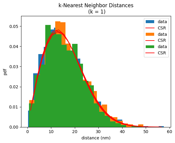
Visualize the combined results

[pipe.meta for pipe in pipes]

[identifier: "1"
 method {
   name: "Pipeline"
   parameter: "{\'computation\': <function computation at 0x7fa4bfe9efc0>, \'file\': <locan.data.locdata.LocData object at 0x7fa4bfeb3890>, \'seed\': SeedSequence(\n    entropy=333947175116642173729758860773302131004,\n    spawn_key=(0,),\n)}"
 }
 creation_time {
   seconds: 1710414571
   nanos: 809359000
 },
 identifier: "1"
 method {
   name: "Pipeline"
   parameter: "{\'computation\': <function computation at 0x7fcc5171efc0>, \'file\': <locan.data.locdata.LocData object at 0x7fcc246f2b50>, \'seed\': SeedSequence(\n    entropy=333947175116642173729758860773302131004,\n    spawn_key=(1,),\n)}"
 }
 creation_time {
   seconds: 1710414571
   nanos: 888556000
 },
 identifier: "1"
 method {
   name: "Pipeline"
   parameter: "{\'computation\': <function computation at 0x7fa4bfe9efc0>, \'file\': <locan.data.locdata.LocData object at 0x7fa3f1be3b10>, \'seed\': SeedSequence(\n    entropy=333947175116642173729758860773302131004,\n    spawn_key=(2,),\n)}"
 }
 creation_time {
   seconds: 1710414571
   nanos: 837072000
 }]

fig, ax = plt.subplots(nrows=1, ncols=1)
for pipe in pipes:
    pipe.nn.hist(ax=ax)
plt.show()