Tutorial about analyzing blink statistics

SMLM depends critically on the fluorescence intermittency or, in other words, the blinking of fluorescence dyes. To characterize blinking properties you can compute on- and off-periods from clustered localizations assuming that they originate from the same fluorophore.

from pathlib import Path

%matplotlib inline

import numpy as np
import matplotlib.pyplot as plt
import scipy.stats as stats

import locan as lc

lc.show_versions(system=False, dependencies=False, verbose=False)

Locan:
   version: 0.22.0.dev32+g4bfc3ab8b

Python:
   version: 3.11.14

Synthetic data

We use synthetic data that represents localizations from a single fluorophore being normal distributed in space and emitting at a constant intensity. We assume that the on- and off-times in units of frames are distributed like a geometric distribution with a mean on_period mean_on and a mean off_period mean_off. Typically a geometric distribution is parameterized by a variable p with p = 1 / mean.

rng = np.random.default_rng(seed=1)

n_samples = 10_000
mean_on = 5
mean_off = 20

on_periods = stats.geom.rvs(p=1/mean_on, size=n_samples, random_state=rng)
off_periods = stats.geom.rvs(p=1/mean_off, size=n_samples, random_state=rng)

On- and off-times are converted in a series of frame numbers at which a localization was detected.

def periods_to_frames(on_periods, off_periods):
    """
    Convert on- and off-periods into a series of increasing frame values.
    """
    on_frames = np.arange(np.sum(on_periods))
    cumsums = np.r_[0, np.cumsum(off_periods)[:-1]]
    add_on = np.repeat(cumsums, on_periods)
    frames = on_frames + add_on
    return frames[:len(on_periods)]

frames = periods_to_frames(on_periods, off_periods)

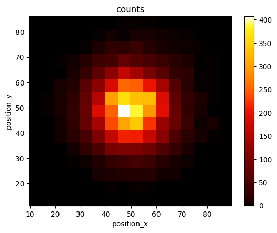
offspring = [rng.normal(loc=0, scale=10, size=(n_samples, 2))]
locdata = lc.simulate_cluster(centers=[(50, 50)], region=[(0, 100), (0, 100)], offspring=offspring, clip=False, shuffle=False, seed=rng)
locdata.dataframe['intensity'] = 1
locdata.dataframe['frame'] = frames

locdata = lc.LocData.from_dataframe(dataframe=locdata.data)

print('Data head:')
print(locdata.data.head(), '\n')
print('Summary:')
locdata.print_summary()
print('Properties:')
print(locdata.properties)

Jupyter environment detected. Enabling Open3D WebVisualizer.
[Open3D INFO] WebRTC GUI backend enabled.
[Open3D INFO] WebRTCWindowSystem: HTTP handshake server disabled.

Data head:
   position_x  position_y  cluster_label  intensity  frame
0   50.507149   36.698297              0          1      0
1   44.539062   27.969248              0          1      1
2   56.876954   42.152826              0          1      2
3   38.878363   43.999842              0          1      3
4   61.001644   54.231150              0          1      4 

Summary:
identifier: "2"
comment: ""
source: DESIGN
state: RAW
element_count: 10000
frame_count: 10000
creation_time {
  2026-04-30T08:33:17.171062Z
}

Properties:
{'localization_count': 10000, 'position_x': np.float64(49.986893963647944), 'uncertainty_x': np.float64(0.09881426457266232), 'position_y': np.float64(49.84659129517861), 'uncertainty_y': np.float64(0.10007238629130723), 'intensity': np.int64(10000), 'frame': np.int64(0), 'region_measure_bb': np.float64(6466.041774468444), 'localization_density_bb': np.float64(1.5465411992056104), 'subregion_measure_bb': np.float64(322.0177777257221)}

lc.render_2d(locdata, bin_size=5);

Blinking statistics

To determine on- and off-times for the observed blink events use the analysis class BlinkStatistics.

bs = lc.BlinkStatistics(memory=0, remove_heading_off_periods=False).compute(locdata)
bs

BlinkStatistics(memory=0, remove_heading_off_periods=False)

bs.results.keys()

dict_keys(['on_periods', 'on_periods_frame', 'off_periods', 'off_periods_frame', 'on_periods_indices'])

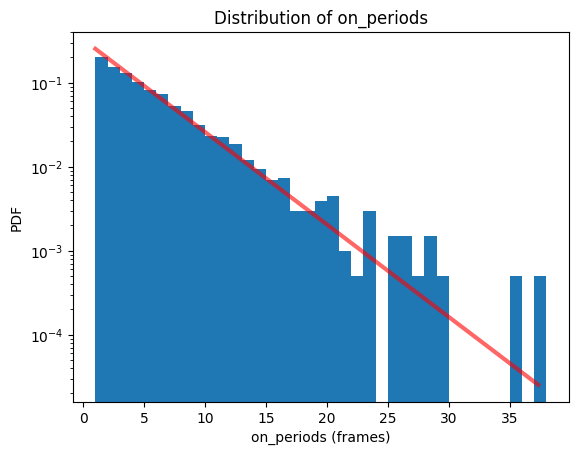
When plotting the histogram an exponential distribution is fitted by default.

bs.hist(data_identifier='on_periods');

bs.hist(data_identifier='off_periods');

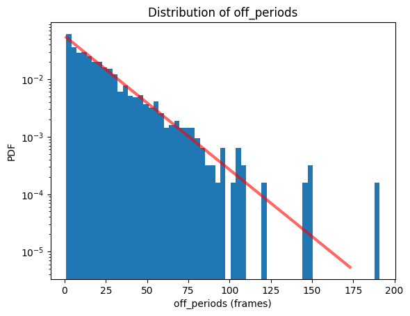
bs.distribution_statistics

{'on_periods': _DistributionFits(analysis_class=BlinkStatistics, distribution=expon_gen, data_identifier=on_periods),
 'off_periods': _DistributionFits(analysis_class=BlinkStatistics, distribution=expon_gen, data_identifier=off_periods)}

The fit results provide loc and scale parameter (see scipy.stats documentation). For loc = 0, scale describes the mean of the distribution..

bs.distribution_statistics['on_periods'].parameter_dict()

{'on_periods_loc': 1.0, 'on_periods_scale': 3.9455984174085064}

bs.distribution_statistics['off_periods'].parameter_dict()

{'off_periods_loc': 1.0, 'off_periods_scale': 18.682830282038594}

Due to the default setting for the scaling parameter loc the mean on_period is on_periods_scale + on_periods_loc in agreement with our input value.

Geometric distribution

We can compare this with a geometric distribution that is estimated from the observed mean on_period on_periods_mean.

on_periods_mean = bs.results['on_periods'].mean()
on_periods_mean.round(2)

np.float64(4.95)

off_periods_mean = bs.results['off_periods'].mean()
off_periods_mean.round(2)

np.float64(19.68)

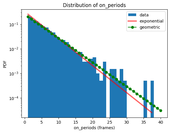
# test result
x = np.arange(stats.geom.ppf(0.01, 1/on_periods_mean), stats.geom.ppf(0.9999, 1/on_periods_mean))
y = stats.geom.pmf(x, 1/on_periods_mean)
fig, ax = plt.subplots()
bs.hist(data_identifier='on_periods', fit=False, label='data')
bs.distribution_statistics['on_periods'].plot(label='exponential')
ax.plot(x, y, '-go', label='geometric')
ax.set_yscale('log')
ax.legend(loc='best')
plt.show()